Understanding Artificial Neural Networks with Hands-on Experience - Part 4. Optimization and Optimizers with Custom Implementations and A Case Study
This post is the 4th part of the series.
- Matrix Multiplication, Its Gradients and Custom Implementations
- Convolution, Its Gradients and Custom Implementations
- Transposed Convolution and Custom Implementations
- Optimization and optimizers with Custom Implementations and A Case Study (this post)
- Hyper-Parameter Learning Rate and Schedulers
In the previous posts, we have been continuously focused on gradients and backpropagation, which is the most important and also most difficult part of understanding neural network principles. With that being covered, we are moving to another important topic – optimization. More specifically, we will talk about fundamentals of optimization and several widely used optimizers, and then use a case study to demonstrate how to implement and use them in a network. For your convenience, this post is organized into the following sections.
- Optimization in neural networks
- Widely used optimizers
- Gradient descent algorithm
- Stochastic gradient descent algorithm
- Gradient descent with momentum algorithm
- RMSprop optimizer algorithm
- Adam optimizer algorithm
- A case study – Regression of Earth-to-Mars transfer orbit
- Implementations of the network and optimizers
- Hyper-parameters and learn rate scheduler*
- Summary
- References
1. Optimization in neural networks
Artificial neural networks are really about training learnable parameters, but how? Figure 1 shows typical steps in an iteration of the training process.
- Step 1 (forward-propagation): Take a new batch of input data, run it through the entire network with current learnable parameters, and compute the output.
- Step 2 (loss): Compute loss using the pre-defined loss function. The whole point of loss is to quantify the errors of the output from the network model against the labels (ground truth) and how well the so-far learnt parameters are doing on the training set. The loss function tells what types of errors you care about and what types of constraints you want to apply to the training. We can have a separate talk about this topic.
- Step 3 (back-propagation): Use the chain rule to compute gradients of the loss with respect to every learnable parameter, for example, the weights and bias used in convolution, transposed convolution, batch-norm as we already covered before.
- Step 4 (optimization): based on the gradients, apply the optimization algorithms to change the learnable parameters a little bit so that the new set of parameters will lead to a decrease in loss (or errors).
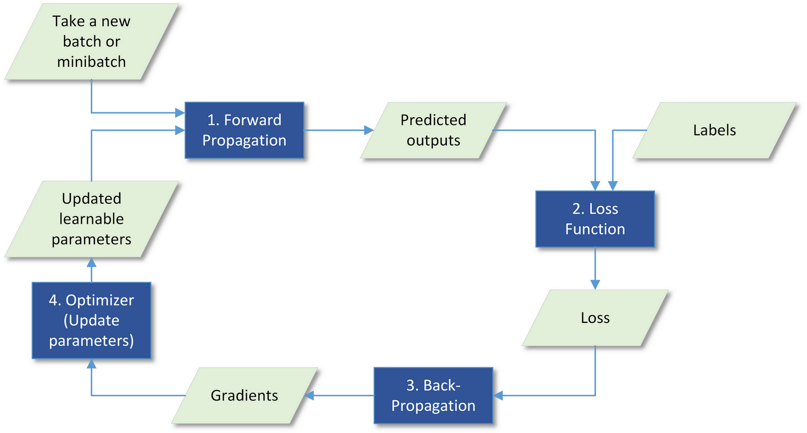
Figure 1 Illustration of the 4 core steps in one iteration of artificial neural networks training.
Repeat Steps 1 through 4 for another batch, then another one. Eventually, you can reach the minimum of the loss function and it means you have optimized the network. This process is also referred to as minimization of the loss function.
2. Widely used optimizers
Various algorithms have been developed for the minimization task. In this section, we will discuss 5 popular optimizers (namely Gradient descent, Stochastic gradient descent, Gradient descent with momentum, RMSprop and Adam) and see how these algorithms are used to train the learnable parameters on the training set.
2.1. Gradient descent
Gradient descent[1] represents the iterative algorithm that changes the learnable parameters by taking a small step in the opposite direction of the gradient of the loss function at the current point (of the learnable parameters). Since gradient points to the direction of steepest increase in the loss, the opposite direction gives the steepest decrease in the loss. That’s why it is called gradient descent.
The basic idea of gradient descent is illustrated in Figure 2 for a contour plot of loss function, \(L\), as a function of two learnable parameters, \({W_a}\) and \({W_b}\). In this plot, red color indicates greater loss and blue color indicates less loss. The minimum loss is indicated with the yellow dot, located at \(\left( { {W_a} = 1.26,{W_b} = 1.23 } \right)\). The initial random estimate of \(\left( { {W_a}^{\left( 0 \right)},{W_b}^{\left( 0 \right)} } \right)\) is indicated by the blue dot close to the top-left corner. The green arrows form a path from the initial point to the minimum loss point. Each arrow represents a training step, which points to the opposite direction of the gradients at the location of that step. For example, consider the 1st step at the blue dot, the gradient of the loss at that location actually points to the left, therefore, the training step takes the direction to the right, towards to the local minimum of loss. The same logic applies to the other steps and it ends up reaching the minimum loss at the yellow dot.
To help understand the intuition behind gradient descent, people often imagine this scenario: a person gets lost in a foggy mountain and is trying to get down to the village in the valley. Because of the fog, he cannot see a direct downhill path to the valley. One solution is to evaluate slope at each step and go with the direction of the steepest descent at the current location. Repeatedly carrying out the same strategy will eventually bring him down to the valley.
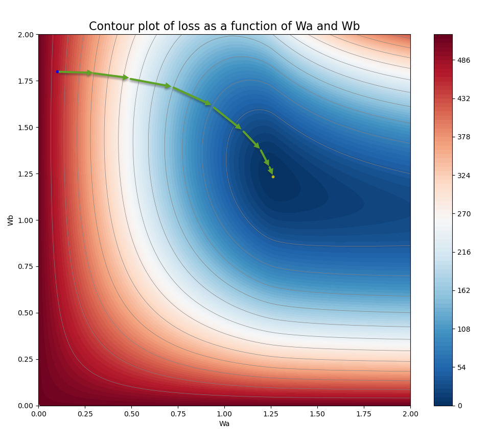
Figure 2 Illustration of gradient descent in an example of loss function with 2 learnable parameters.
Mathematically, let’s consider a regression case: the training dataset contains \(N\) separate samples, where the input of the \(i\)-th sample is \({X_i}\) and its target is \({Y_i}\), and the network has \(M\) learnable parameters \(\left( { {w_1}, \cdots ,{w_M} } \right)\). The predicted output \({\hat Y_i}\) from the network for each sample can be written as
A typical loss function can be defined as Mean Squared Error
Also assume that the gradient (or partial derivative) of the loss function \(L\left( { {w_1}, \cdots ,{w_M} } \right)\) w.r.t. individual parameter \({w_m}\) has already been computed from back-propagation using the current values of the parameters \(\left( { {w_1}, \cdots ,{w_M} } \right)\), and labelled as \({g_m}\)
Then, the iterative algorithm of gradient descent to update the learnable parameters can be written as
where \(t\) denotes the \(t\)-th iteration of update, \(\alpha \) is a positive number and denotes the learning rate and controls how big a step to take on each iteration.
There are a few points to make about Equation (4).
- The term \( - \alpha \cdot {g_m}\) is the amount to adjust \({w_n}\). The negative sign in the equation indicates taking the opposite direction of the gradient.
- If the gradient \({g_m}\) is positive, it means that an increase in \({w_n}\) will lead to an increase in loss \(L\). In this case, the adjustment amount \( - \alpha \cdot {g_m}\) will be negative, so the new \({w_m}\) will be smaller, which in turn will cause the loss to be smaller. Vice versa.
- To differentiate from the learnable parameters \(w\), the learning rate \(\alpha \) is called hyper-parameter and typically requires users to tune up instead of learning from training. In other words, users need to try different \(\alpha \) in order to find an optimal one to use.
- Gradient descent typically uses the entire dataset as a batch to pass through the network, then performs one update of the learnable parameters. This is referred to as one “epoch” in training.
2.2. Stochastic gradient descent
Stochastic gradient descent (SGD) [2] is a variant of gradient descent and share the same basic idea and equations with GD. The only major difference is that, unlike GD that updates the parameters only once in an epoch based on the entire training dataset, SGD performs an update after each individual training sample passes through the network. Typically, the training dataset is randomly shuffled, and thus the update is based on a randomly picked sample, that’s why it is called Stochastic gradient descent - Stochastic means “random”.
The tradition gradient descent can be thought as to have a batch containing the entire training samples, while SGD can be thought as to have a batch contain only one single sample for each update. What’s the impact of this difference? In general, SGD is more aggressive in updating the parameters and it provides the chance to converge faster for the same number of epochs, at least in the early epochs. However, due to the noise or errors in training dataset, update based on a single sample can have big bias. For example, even for the same set of parameters \(\left( { {w_1}, \cdots ,{w_M} } \right)\), two different training samples can lead to opposite directions in how to change the parameters. The fortunately thing is that, while some samples might cause the parameter to go with “wrong way”, other samples might cancel it out, so the overall trend still goes to the right way. On the contrary, gradient descent update the parameters at a much slower pace, but a much smoother way to find the optimal solution. It’s worth mentioning one burden about GD: if the entire dataset is passed through the network, it requires significantly more computing resources such as GPU memory.
A tradeoff between GD and SGD is introduced to neural networks by using “mini-batch” that takes a randomly-shuffled subset of the dataset instead of the entire dataset for each update. People usually choose a mini-batch size of power of 2. Now traditional GD and SGD can be thought of as two special and extreme cases of a more general mini-batch gradient descent.
Figure 3 compares the behaviors of 4 different mini-batch configurations by plotting loss vs epochs during training. In this example, the dataset contains 512 samples. The 4 configurations diffs only in the size of mini-batch: Mini-batch size=1, so 512 updates per epoch (SGD); Mini-batch size=32, so 16 updates per epoch; Mini-batch size=512, so 1 update per epoch (GD); Hybrid, mini-batch size of 32 for the first 8 epochs and size of 512 for the rest. Each point on the plots represents one evaluation of loss upon one update. For small min-batch size (such as 1), there are too many points, which would make the plots too busy, therefore it only plots 1 out of every 32 points for the case of mini-batch size=1 and 1 out of every 2 points for the case of mini-batch size=32.
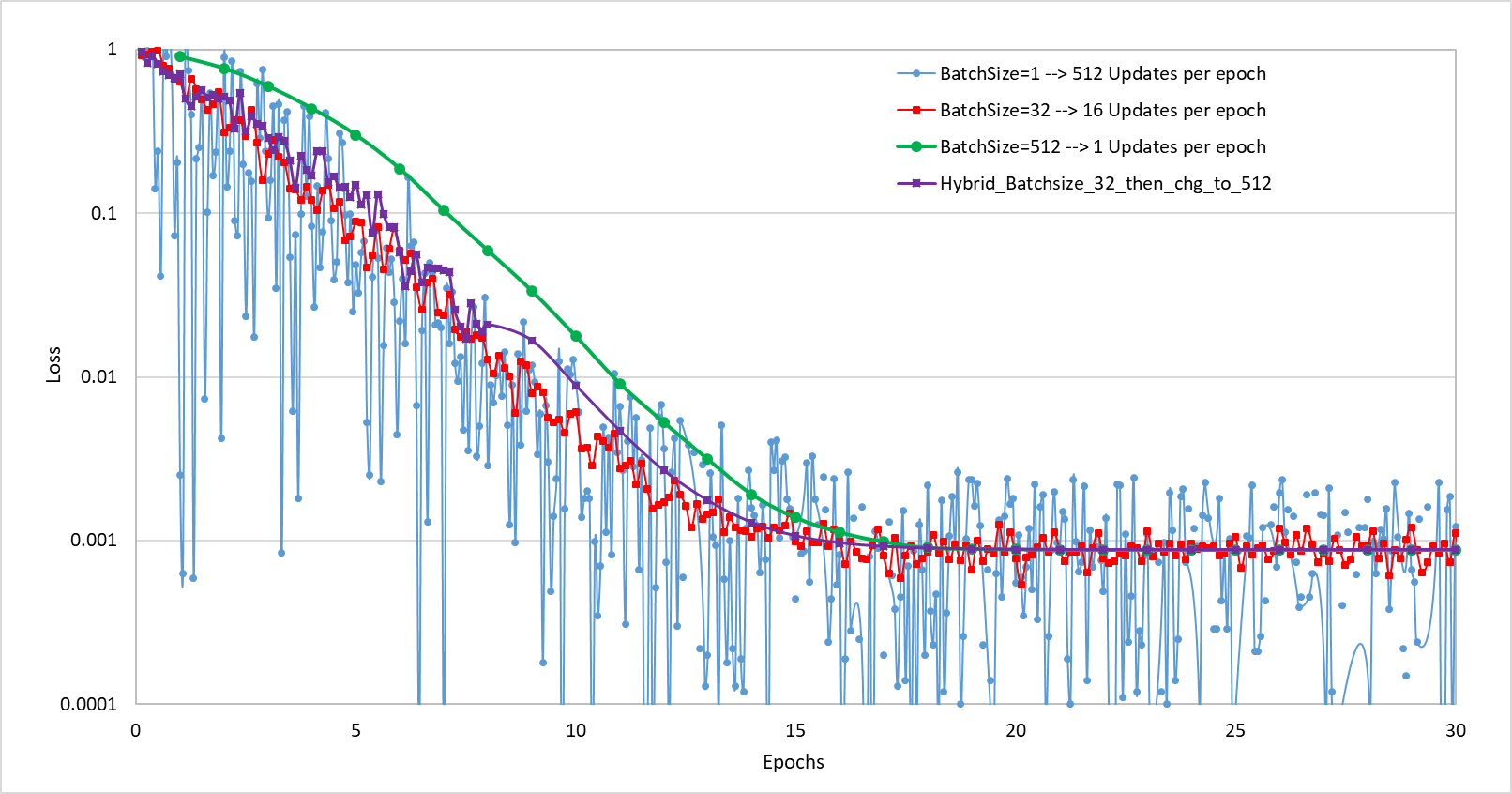
Figure 3 Comparison of the impact of batch size on gradient descent.
From the plots, we can see that \(batchsize = 512\) has a slower converge at the early epochs, but the converge is quite smooth and stable. On the contrary, \(batchsize = 32\) has a faster converge during the early epoch, but suffers from noise. That’s why the hybrid configuration is investigated as well, trying to combine the advantages from both configurations.
2.3. Gradient Descent with momentut
Gradient descent with momentum[3] is a GD-based algorithm developed to speed up training by accelerating updates in the “right” direction and dampen oscillations in other directions. The basic idea is to compute an exponentially weighted average of the gradients from both the current step and the previous steps and then use that average to update the learnable parameters. Mathematically, it can be written as
\({v_m}^{\left( t \right)} = \beta \cdot {v_m}^{\left( {t - 1} \right)} + \left( {1 - \beta } \right) \cdot {g_m}^{\left( t \right)}\) (5)
\({w_m}^{\left( {t + 1} \right)} = {w_m}^{\left( t \right)} - \alpha \cdot {v_m}^{\left( t \right)}\) (6)
with the initial \({v_m}^{\left( 0 \right)}\)=0 and \(\beta \in \left[ {0,1} \right)\). Let’s understand the meaning of Equation (5). If we substitute \({v_m}^{\left( {t - 1} \right)}\) with \({v_m}^{\left( {t - 2} \right)}\) and \({g_m}^{\left( {t - 1} \right)}\) and keep doing it recursively, it will end up with
Equation (7) indicates that \({v_m}^{\left( t \right)}\) is a sum of past gradients \({g_m}^{\left( k \right)}\) weighted by the exponential factor of \({\beta ^{t - k}}\). That’s why it is called exponentially weighted average of the gradients. Because \(\beta \) is smaller than \(1\), an older gradient has less contribution to \({v_m}^{\left( t \right)}\) than a newer gradient.
The weighted average can be thought of as the momentum of a moving object in physics that has an inertia to main the motion in the original direction. The concept can be illustrated in Figure 4. When the “history” gradients are not taken into consideration in the standard GD algorithm, update is purely based on the “current” location alone and the path could look like the oscillating red arrows. By using the exponentially weighted average of the “history” in gradient descent with momentum, the components in the horizontal direction are likely to cancel out partially. As a result, the oscillations is reduced and the net effect is that the learning is making more progress in the vertical direction (the yellow arrow).
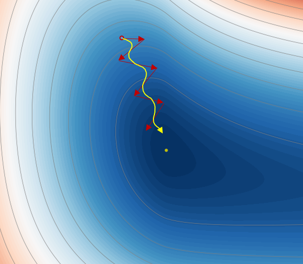
Figure 4 Illustration of the concept of gradient descent with momentum.
Please note that, if \({v_m}^{\left( 0 \right)}\) is set to zero, \({v_m}^{\left( t \right)}\) from Equation (5) will have a bias for early steps. To compensate for this bias, \({v_m}^{\left( t \right)}\) is adjusted with a correction factor before being used in Equation (6):
However, the bias becomes less important when \(t\) becomes bigger. Therefore, this correction is ignored in some implementations.
A commonly used value for \(\beta \) is \(0.9\). When \(\beta = 0\), this algorithm returns back to the standard GD algorithm.2.4. RMSprop
RMSprop stands for root mean square propagation[4]. It is another algorithm to dampen undesired oscillations by making the learning rate adaptive to the exponentially weighted average of the squared gradients from the past steps.
\({s_m}^{\left( t \right)} = \beta \cdot {s_m}^{\left( {t - 1} \right)} + \left( {1 - \beta } \right) \cdot {\left( { {g_m}^{\left( t \right)} } \right)^2}\) (9)
\({w_m}^{\left( {t + 1} \right)} = {w_m}^{\left( t \right)} - \frac{\alpha }{ {\sqrt { {s_m}^{\left( t \right)} } + \epsilon} } \cdot {g_m}^{\left( t \right)}\) (10)
The difference between Equations (9) and (5) is that it is the squared gradients, instead of the gradients, used to compute the weighted average for RMSprop. Comparing Equation (10) to Equation (4), we can see the only difference is that the learning rate \(\alpha \) is adjusted as \(\frac{\alpha }{ {\sqrt { {s_m}^{\left( t \right)} } + \epsilon } }\), referred to as effective learning rate. A tiny number \( \epsilon \) is used to avoid the divided-by-zero exception where \({s_m}^{\left( t \right)} = 0\). A commonly used value for \(\beta \) is \(0.99\).
The intuition behind RMSprop is illustrated in Figure 5 below, a contour plot of loss as a function of two learnable parameters, \({w_h}\) in horizontal direction and \({w_v}\) in vertical direction. The starting point is A and the target point is M, the minimum location of the loss. In this example, we want to slow down the learning in the vertical direction and (relatively) speed up learning in the horizontal direction. Let’s see how the RMSprop algorithm help accomplish this objective. At point A, the magnitude of the gradient in the vertical direction, \({g_v}\), is much larger than that in the horizontal direction, \({g_h}\) (as you can see from the contour, the change in loss at point A is much more dramatic in the vertical direction). As a result, \({s_v}\) is much larger than \({s_h}\), so \(\frac{1}{ {\sqrt { {s_v} } } }\) is much smaller than \(\frac{1}{ {\sqrt { {s_h} } } }\). Therefore, the effective learning rate in the vertical, \(\frac{\alpha }{ {\sqrt { {s_v} } } }\), is smaller than that in the horizontal direction, \(\frac{\alpha }{ {\sqrt { {s_h} } } }\). The net effect is that the oscillation in the vertical direction is reduced and the training update will end up looking more like the yellow curve.
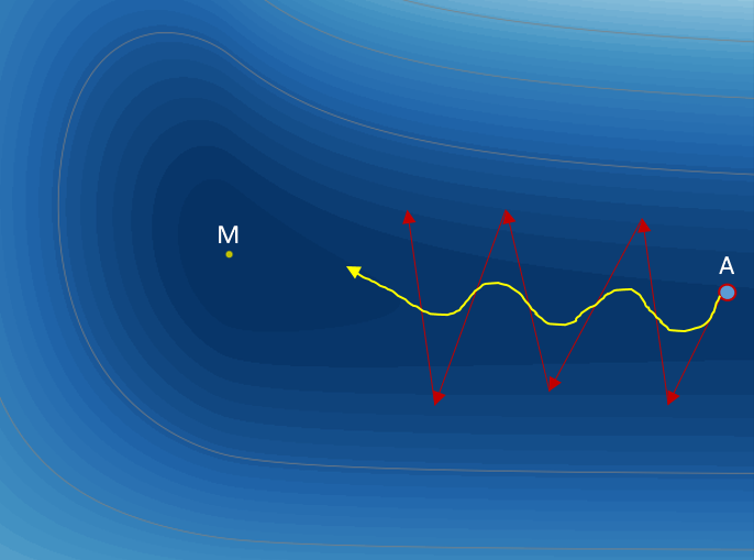
Figure 5 Illustration of the concept of RMSprop.
2.5. Adam
Adam[5] is another optimization algorithm that has been shown to work very well on a wide variety of applications. Adam stands for adaptive moment estimation. It combines the advantage of the gradient descent with momentum algorithm together with that of the RMSprop algorithm
\({v_m}^{\left( t \right)} = {\beta _1} \cdot {v_m}^{\left( {t - 1} \right)} + \left( {1 - {\beta _1} } \right) \cdot {g_m}^{\left( t \right)}\) (11)
\({v_m}^{\left( t \right)} := \frac{ { {v_m}^{\left( t \right)} } }{ {1 - {\beta _1}^t} }\) (12)
\({s_m}^{\left( t \right)} = {\beta _2} \cdot {s_m}^{\left( {t - 1} \right)} + \left( {1 - {\beta _2} } \right) \cdot {\left( { {g_m}^{\left( t \right)} } \right)^2}\) (13)
\({s_m}^{\left( t \right)} := \frac{ { {s_m}^{\left( t \right)} } }{ {1 - {\beta _2}^t} }\) (14)
\({w_m}^{\left( {t + 1} \right)} = {w_m}^{\left( t \right)} - \frac{\alpha }{ {\sqrt { {s_m}^{\left( t \right)} } + \epsilon} } \cdot {v_m}^{\left( t \right)}\) (15)
Comparing these equations with those in the previous sections, we can see that Equations (11), (12) and the term \({v_m}^{\left( t \right)}\) in Equation (15) correspond to the momentum algorithm, whereas Equations (13), (14) and the adaptive learning rate \(\frac{\alpha }{ {\sqrt { {s_m}^{\left( t \right)} } + \epsilon} }\) in Equation (15) correspond to the RMSprop algorithm.
There are 3 hyper-parameters in Adam algorithm. \({\beta _1}\) and \({\beta _2}\) are for the exponential weighted average of gradient and squared gradient, respectively. Typical default values are \(0.9\) for \({\beta _1}\) and \(0.99\) for \({\beta _2}\) and works well in most scenarios. On the other hand, the learning rate \(\alpha \) typically requires tune-up to find the optimal value for individual applications.
3. A case study – Regression of Earth-to-Mars transfer orbit
Just about two weeks ago, NASA’s Perseverance Rover successfully landed on Mars after its half a year and \(292.5\) million-mile journey from our planet, the Earth. Inspired by this great accomplishment, we will use a simplified model of the Earth-to-Mars transfer orbit as an example to demonstrate how to implement the optimization algorithms and how to incorporate them into neural network to help solve regress tasks.
With approximation (please see Figure 6), let’s assume both Earth (on blue circle) and Mars (on red circle) are moving around the Sun in circular orbits. Their radii are \(1.0\) \(AU\) and \(1.5237\) \(AU\), respectively (\(AU\) is astronomical unit, roughly the distance from Earth to the Sun and equal to about \(150\) million kilometers). In this story (somewhat different from the Perseverance rover), a spacecraft is launch from Earth at the point marked by the blue dot, then travels along Hofmann Transfer Orbit, and finally reaches Mars orbit at the point marked by the red dot. The Hofmann Transfer Orbit (green solid curve in the figure) is an elliptical orbit around the Sun and requires least amount of propellant to reach Mars. BTW, the actual orbit of Perseverance Rover is a little bit different from the Hofmann Transfer Orbit and takes less time to reach Mars. We will write a separate post to animate the Hofmann Transfer Orbit.
Taking the center of the Sun as the origin of the coordinate system, the Hofmann Transfer Orbit can be described by the elliptical equation
where \(A = 1.261845\) is the length of semi-major axis and \(B = 1.234378\) is the length of semi-minor axis in unit of \(AU\). The offset of \(0.26185\) in x-axis is half of the distance between the two foci. This offset shows up in Equation (16) because the origin of the coordinate system is chosen to be at the center of the Sun (one of the two foci) instead of the center of the ellipse.
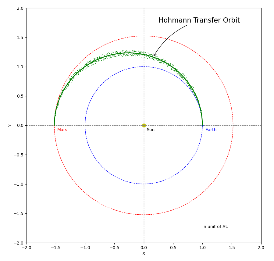
Figure 6 Illustration of the Earth-to-Mars Transfer orbit.
Using Equation (16), we sampled \(512\) \(\left( {N = 512} \right)\) points \(\left( { {X_i},{Y_i} } \right)\) of the Hohmann Transfer Orbit and then added random noise to the samples. The \(512\) samples are shown as the green dots in Figure 6.
Now the task is, given the \(512\) samples and Equation (16) of an ellipse with unknown parameters \(A\) and \(B\), to find out what the values of \(A\) and \(B\) should be. This is a typical regress problem and can be solved using various mathematical ways. In this post, we will use neural networks with the discussed optimization algorithms to solve the problem. For the purpose of demonstration, we will assume the parameters \(A\) and \(B\) are independent, so the networks will have two learnable parameters, one for \(A\) and the other one for \(B\).
4. Implementations of the network and optimizers
Recall that a typical network consists of 4 key steps during one iteration: forward propagation, calculation of loss, backpropagation and optimization. We will manually build each of these components. In this example, the learnable parameters are named \({w_A}\) and \({w_B}\), representing \(A\) and \(B\) respectively. They can be initialized with random numbers or with specific values for experiments.
4.1. Custom Dataset and Dataloader
To prepare the data for training, we write code to build our custom dataset by subclassing torch.utils.data.Dataset and implementing 3 member functions:
class EllipseDataset(torch.utils.data.Dataset):
    def __init__(self, N, A, B, noise_scale=0.1, transform=None):
        ...

    def __len__(self):
        ...

    def __getitem__(self, idx):
        ...
Inside the __init__ constructor, it calls generate_training_data(N, a, b, noise_scale=0.1, plot_data=True) to generate the training dataset of \(512\) samples of \(\left( { {X_i},{Y_i} } \right)\). In addition, transform can be very convenient when some operations such as transformation, scaling, image crop, etc. need to be applied to the samples. In this example, there is no such a need, so it is set to None. Please see the detailed source code here on GitHub.
Here are the two lines to instantiate EllipseDataset and Dataloader, and then fetch the mini-batch data from the Dataloader during the training loop.
xy_dataset = EllipseDataset(nsamples, a, b, noise_scale=0.1, transform =None)
xy_dataloader = DataLoader(xy_dataset, batch_size=batch_size, shuffle=True, num_workers=0)
...
for t in range(epoch):
    for i_batch, sample_batched in enumerate(xy_dataloader):
        x, y = sample_batched['x'], sample_batched['y']
        ...
The argument batch_size can be any integer between \(1\) and \(N\) inclusive, but is suggested to choose a power of \(2\). The vectored \(x\) represents the input features (actually the \(x\)-coordinates of the sampled points from the Hofmann Transfer Orbit) and the vectored \(y\) represents the corresponding targets (the simulated \(y\) -coordinates of the sampled points).
4.2. Forward pass
The forward pass is to calculate the predicted \(\hat y\) for the given input \(x\) based on the following equation, which is simply re-arranged form Equation (16) above.
One thing to note is that, due to the noise introduced to the samples, the subtraction operation can result in negative values that is invalid to take square root. For those samples running into this issue, their out \({\hat y_i}\) are set to zero, and excluded from the loss and gradient calculations.
4.3. Loss function
In this example, loss is defined as the mean squared error between the predicted \({\hat y_i}\) and the given target \({y_i}\).
where \(N'\) denotes the number of all samples in the current mini-batch that don’t run into the square root issue.
4.4. Back-propagation to calculate gradients
The gradients of the loss function w.r.t. the learnable parameters \({w_A}\) and \({w_B}\) are derived using the chain rule that have been extensively discussed in the previous posts. Here we directly give out the derived results.
\(\frac{ {\partial L} }{ {\partial {w_A} } } = \frac{1}{ {N'} }\mathop \sum \limits_{i = 1}^{N'} 2\left( { { {\hat y}_i} - {y_i} } \right) \cdot \frac{ { { {\left( { {x_i} + 0.26185} \right)}^2} } }{ { { {\hat y}_i} } } \cdot \frac{ { {w_B}^2} }{ { {w_A}^3} }\)
\(\frac{ {\partial L} }{ {\partial {w_B} } } = \frac{1}{ {N'} }\mathop \sum \limits_{i = 1}^{N'} 2\left( { { {\hat y}_i} - {y_i} } \right) \cdot \frac{ { { {\hat y}_i} } }{ { {w_B} } }\)
(29)4.5. Update of learnable parameters using the optimizers
The gradient descent, SGD, GD with momentum, RMSprop and Adam are implemented following the equations described in Section 2. In order validate these custom implementations, we also build another block of codes to do the same job using Torch built-in function[6] for comparison. For example, the following snippet shows the implementation of the Adam algorithm.
if flag_manual_implement:
    # Step 3: perform back-propagation and calculate the gradients of loss w.r.t. Wa and Wb
    dWa_via_yi = 2.0 * (y_pred - y) * ((x + c) ** 2) * (Wb ** 2) / (Wa ** 3) / y_pred
    dWa = dWa_via_yi[~negativeloc].mean()  # gradient w.r.t Wa

    dWb_via_yi = (2.0 * (y_pred - y) * y_pred / Wb)
    dWb = dWb_via_yi[~negativeloc].mean()  # gradient w.r.t Wb

    # Step 4: Update weights using the Adam algorithm.
    with torch.no_grad():
        beta1_to_pow_t *= beta1
        beta1_correction = 1.0 - beta1_to_pow_t
        beta2_to_pow_t *= beta2
        beta2_correction = 1.0 - beta2_to_pow_t

        VdWa = beta1 * VdWa + (1.0 - beta1) * dWa
        SdWa = beta2 * SdWa + (1.0 - beta2) * dWa * dWa
        Wa -= learning_rate * (VdWa / beta1_correction) / (torch.sqrt(SdWa) / math.sqrt(beta2_correction) + eps)

        VdWb = beta1 * VdWb + (1.0 - beta1) * dWb
        SdWb = beta2 * SdWb + (1.0 - beta2) * dWb * dWb
        Wb -= learning_rate * (VdWb / beta1_correction) / (torch.sqrt(SdWb) / math.sqrt(beta2_correction) + eps)

else:  # do the same job using Torch built-in autograd and optim
    # reset the gradients of the learnable parameters to zero. Otherwise, it will be accumulated.
    optimizer.zero_grad()
    # Step 3: perform back-propagation and calculate the gradients of loss w.r.t. Wa and Wb
    loss.backward()
    # Step 4: Update weights using Adam algorithm.
    optimizer.step()
Please see the complete source code for GD, GD with momentum, RMSprop and Adam on GitHub, respectively. You can also try the custom implementation or the Torch version by setting flag_manual_implement to True or False.
Figures 7 through 10 shows the results from using the 4 optimizers, respectively. The starting point is \({A_{start} } = 0.1\) and \({B_{start} } = 1.8\). You can see from the figures, all of the 4 final results are very close to the ground truth (\({A_{truth} } = 1.261845\) and \({B_{truth} } = 1.234378\)) that were used to generate the noisy samples. However, each optimizer has its own searching path. Figure 11 shows an animation of the 4 optimizers’ update paths from the starting point to the minimum loss. Please note that this video is not an apple-to-apple comparison between these algorithms because different learning rates and adjustment were used. Why not use exactly the same learning rates and adjustment? It is because a learning rate working for one algorithm could cause failure for another one. We will talk about learning rate in a separate post. The animation is presented here to provide some general ideas. Just in case if the video cannot be played in your browser, you can download the mp4 video here . You can also find the source code of the animation here.
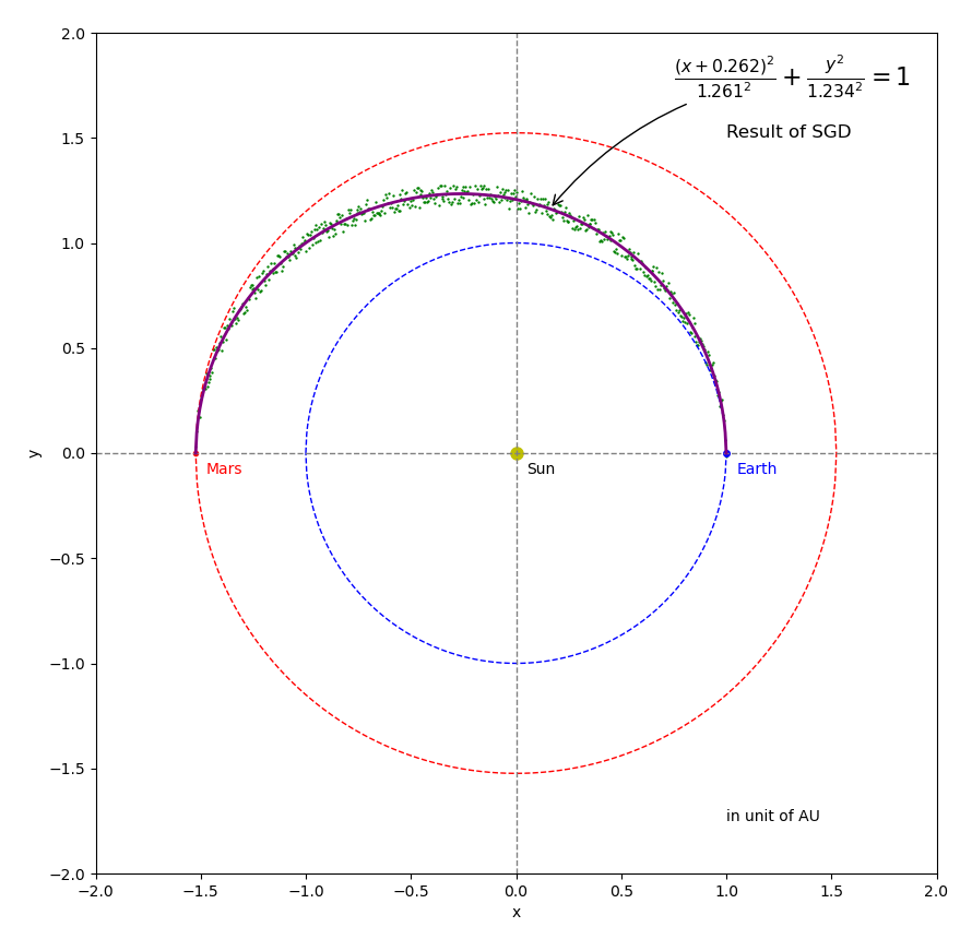
Figure 7 Results of the SGD optimizer.
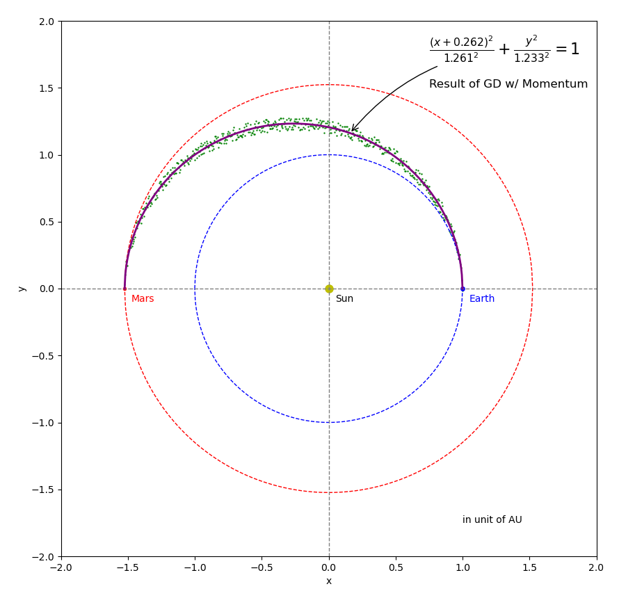
Figure 8 Results of the GD with Momentum optimizer.
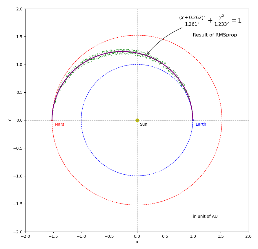
Figure 9 Results of the RMSprop optimizer.
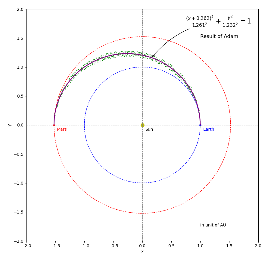
Figure 10 Results of the Adam optimizer.
Figure 11 Animation of the 4 optimizers’ update paths from the starting point to the minimum loss.
5. Hyper-parameters and learn rate scheduler
This post has been quite long and the hyper-parameters and learning rate schedulers seem to deserve a separate post, so we will stop here and will cover those topics separately.
6. Summary
In this post, we went through the fundamentals of optimization in artificial neural networks and discussed 4 widely used optimizers (gradient descent / stochastic gradient descent and its variants to speed up the training using GD with momentum, RMSprop and Adam algorithms). We also demonstrated how to implement them with a network to solve a regression task in the case study of Hohmann Earth-to-Mars Transfer Orbit.
We hope, by walking through these topics and hands-on implementations, we can gain in-depth understanding of how neural network works. Those terminologies, such as gradients, back-propagation, loss function, optimization, etc. will hopefully no longer seem to be a secret.
7. References
- [1] Gradient descent on Wikipedia.
- [2] Léon Bottou (1998). Online Algorithms and Stochastic Approximations.
- [3] Ning Qian (1999). On the momentum term in gradient descent learning algorithms. Neural networks : the official journal of the International Neural Network Society, 12(1):145–151.
- [4] Geoffrey Hinton. Lecture 6e rmsprop: Divide the gradient by a running average of its recent magnitude. (Page 26)
- [5] Diederik P. Kingma and Jimmy Lei Ba (2014). Adam : A method for stochastic optimization.
- [6] torch.optim - PyTorch documentation.