Understanding Artificial Neural Networks with Hands-on Experience - Part 3. Transposed Convolution and Custom Implementations
Time flies. In the last post from September 2020, we discussed convolution for neural networks and how to implement its forward and backward propagations. In this post, we will talk about transposed convolution, the 3rd part of the series.
- Matrix Multiplication, Its Gradients and Custom Implementations
- Convolution, Its Gradients and Custom Implementations
- Transposed Convolution and Custom Implementations (this post)
- Optimization and optimizers with Custom Implementations and A Case Study
- Hyper-Parameter Learning Rate and Schedulers
In a similar way as we did for Convolution in the previous post, we will use the 2-D (for image height and width) scenario as an example to explain the concept of transposed convolution and demonstrate how to implement our own versions, including both forward and backward propagation. The basic ideas can be extended to 1-D and 3-D as well. Here are the outlines of this post.
- Transposed convolution
- Mathematical Operation of Transposed Convolution
- Transposed Convolution Output Size
- The 1st Implementation of ConvTranspose2d (Forward and Backward)
- The 2nd Implementation of ConvTranspose2d
- Validation against Torch Built-ins
- Summary
- References
1. Transposed Convolution
Transposed convolution is an up-sampling method commonly used in CNN networks. For instance, in Autoencoder artificial neural networks[1], the encoder layers reduce input image size using down-sampling and encodes the features in lower resolutions; the decoder layers reconstruct the information back from the reduced encoded size-reduced feature images to the original input size by doing transposed convolution.
Why is it called transposed convolution?
To answer this question, we need to look at convolution again from a different perspective – matrix multiplication. Let’s revisit the example used in the previous post: a \(5 \times 5\) input matrix data convolved with a \(3 \times 3\) kernel with \( stride=1\) and no padding, the convolution output is a \(3 \times 3\) matrix, as shown in Figure 1.
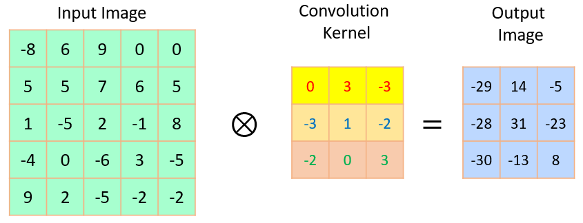
Figure 1 An example of convolution.
If we rearrange (or flatten) the \(5 \times 5\) input matrix into a \(25 \times 1\) column vector, the convolution kernel into a new \(9 \times 25\) transformation matrix, and rearrange the \(3 \times 3\) output matrix into a \(9 \times 1\) column vector, the convolution in Figure 1 is equivalent to a matrix multiplication, as shown in Figure 2. The highlighted color in the transformation matrix indicates how it is built from the given kernel. BTW, please also note that there are a lot of zeros in the sparse transformation, which makes matrix multiplication much less efficient in computation than convolution to achieve the same results. In fact, the number of multiplications in the matrix multiplication way is \(9 \times 25 = 225\), while the number is only \(3 \times 3 \times 3 \times 3 = 81\) for the convolution way. In general, if the input matrix size is \(N \times N\) and the kernel size is \(K \times K\), the ratio of computation burden is about \({N^2}/{K^2}\). When \(N\) is big, the burden becomes significant.
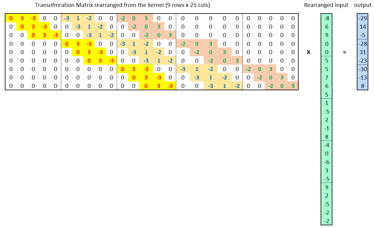
Figure 2 A convolution is equivalent to a matrix multiplication.
However, computation efficiency is not today’s focus. Today’s focus is that you can use convolution to map from the \(5 \times 5\) input matrix (or equivalently \(25 \times 1\) vector) into the \(3 \times 3\) output matrix (or equivalently \(9 \times 1\) vector) in this example, and, similarly, you can also go the other way around and map from the resulting \(3 \times 3\) output matrix back into the original \(5 \times 5\) matrix domain while maintaining the 1-to-9 connectivity relationship of the convolution. How? Use transposed convolution, as illustrated in Figure 3.
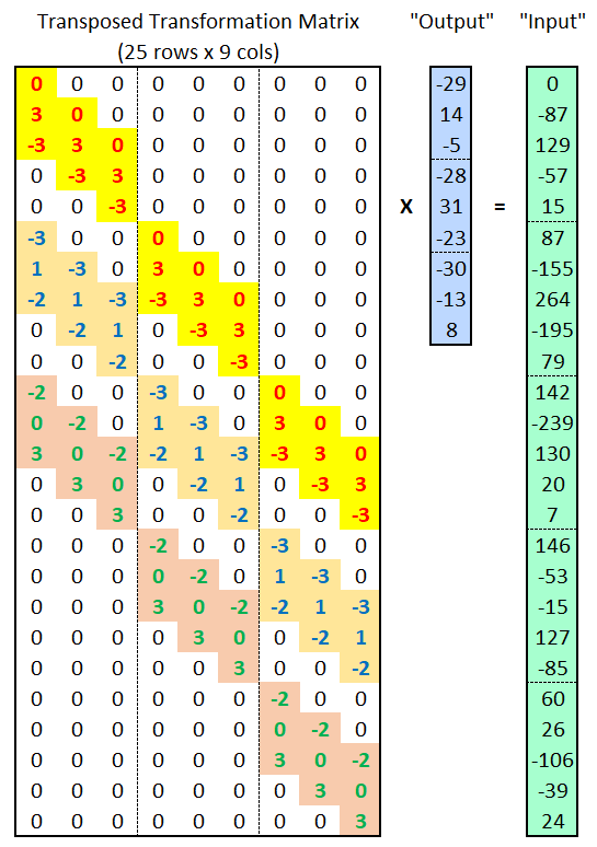
Figure 3 A transposed convolution is equivalent to a transposed matrix multiplication.
The transposed transformation matrix has a size of 25 rows x 9 cols. Multiplying this transposed matrix with the \(9 \times 1\) column vector (flattened from the \(3 \times 3\) output matrix of forward convolution) generates a \(25 \times 1\) vector. Later this \(25 \times 1\) vector can be reshaped into \(5 \times 5\) matrix. This operation is known as transposed convolution. If convolution is thought of as a forward propagation operation, transposed convolution can be thought of as its backward propagation operation. So you might even call it transpose of the original convolution, or backward pass of the original convolution, for easier understanding. However, it must be pointed out that, transposed convolution is not exactly an “inverse” convolution, like FFT⟺iFFT. In other words, transposed convolution reverses only the spatial transformation between input and output, in particular the shape and mapping relationship, but it does not restore the original matrix values.
Again, the transposed matrix multiplication is not computationally efficient because of the filled-in zeros in the sparse transformation matrix. Here we just use matrix multiplication to introduce the concept of transposed convolution. The actual mathematical operation of transposed convolution will be explained later.
It’s also worth mentioning that, in neural networks, one big difference between transposed convolution and other interpolation-based up-sampling techniques is that transposed convolution has learnable parameters (weights and bias) and therefore could lead to optimal upsampling via training.
2. Mathematical Operation of Transposed Convolution
To understand the actual mathematical operation of transposed convolution, we can think of transposed convolution as an associated backward convolution of another forward convolution that has a kernel size of \({N_v} \times {N_u}\), padding of \({P_x}\) and \({P_y}\), and stride of \({S_x}\) and \({S_y}\), along the horizontal and vertical directions, respectively. The forward convolution maps from an input size \({N_{xIn}} \times {N_{yIn}}\) into an output size \({N_{xOut}} \times {N_{yOut}}\). In this section, we will explore how the transposed convolution maps from the output size \({N_{xOut}} \times {N_{yOut}}\) back into original size \({N_{xIn}} \times {N_{yIn}}\).
2.1. Distribution view of ConvTranspose2d
Without loss of generality, let’s consider an example of 2D “forward” convolution: a \(5 \times 5\) input matrix (referred to as \(conv\_input\) ) convolved with two \(3 \times 3\) kernel (referred to as \(conv\_kernel\) ) using \(padding=1\) and \(stride=2\), and generates two channels of \(3 \times 3\) output matrices, referred to as \({conv\_output}\). The task for its associated transposed convolution is to transform from the two \({conv\_output}\) matrices back to the \(conv\_input\) domain. Let’s assume the \({conv\_output}\) matrices to serve as the input of the transposed convolution (also referred to as \({tc\_input}\)) are
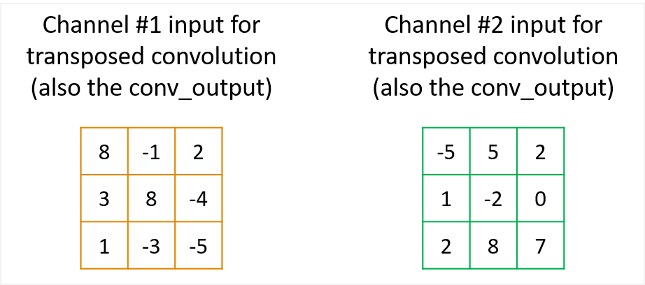
Figure 4 Example of the input matices for the \(associated\) transposed convolution, which come from the output of the “forward” convolution.
And the two kernels of the transposed convolution, referred to as \(tc\_kernel\), are

Figure 5 The two kernels of the associated transposed convolution.
Figures 6 and 7 illustrate how the 1st two elements in the \({tc\_input}\) are distributed back to the “original” \(conv\_input\) \(5 \times 5\) matrix domain via the transposed convolution operation. The other elements are handled in the same way. Please note a few things in the illustration.
- Each element in \({tc\_input}\) contributes back to a total of \(3 \times 3\)=9 elements of original \(conv\_input\) space via the \(3 \times 3\) \(tc\_kernels\).
- Because \(padding=1\) was used in the “original” forward convolution, each border of the intermediate matrix in the \({tc\_output}\) space (the 3rd column in the figures) is also padded by 1 during the mapping in the transposed convolution.
- Because \(stride=2\) was used in the forward convolution, the mapping in the transposed convolution also jump by 2 over the \({tc\_input}\) space.
- Individual channels are processed separately and then summed elementwise to give the corresponding output channel results of the final \({tc\_output}\).
This 1-to-9 mapping pattern (including padding and stride) maintains the original 9-to-1 relationship in the forward convolution. Animation in Figure 8 illustrates the complete operations of this transposed convolution example.
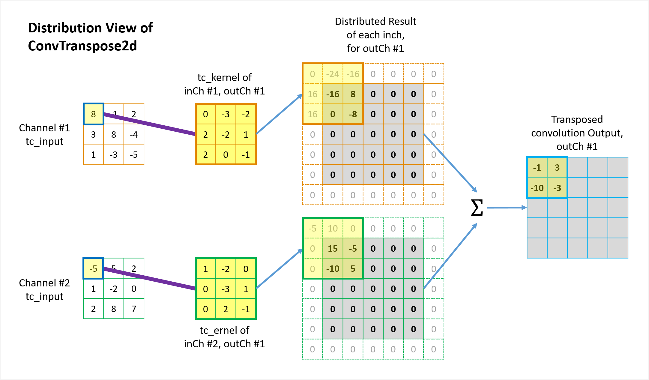
Figure 6 Illustration of how the 1st element in the tc-input distrbutes back to the \({tc\_output}\) from distrbution view of transposed convolution.
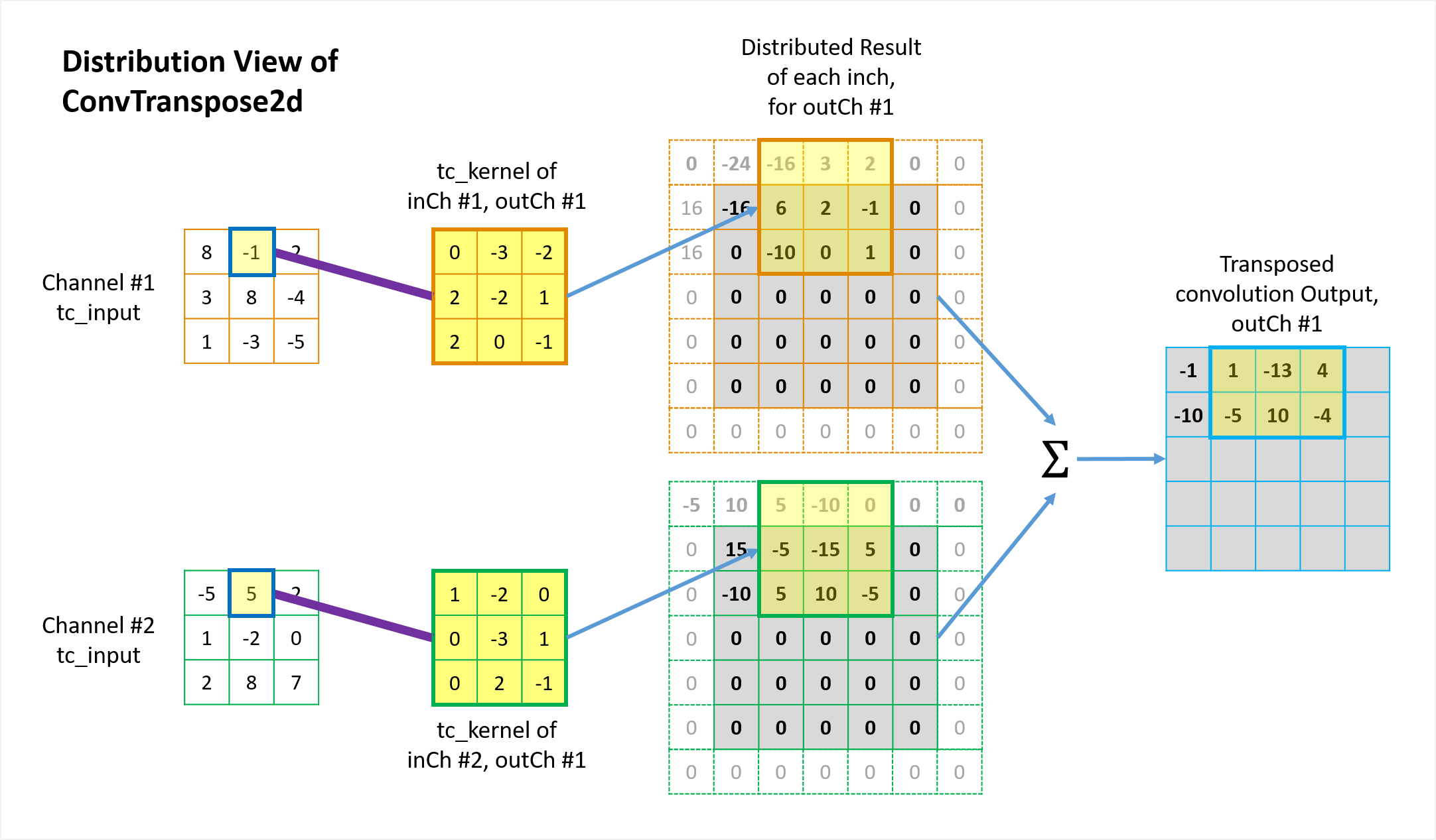
Figure 7 Illustration of how the 2nd element in the tc-input distrbutes back to the \({tc\_output}\) from distrbution view of transposed convolution.
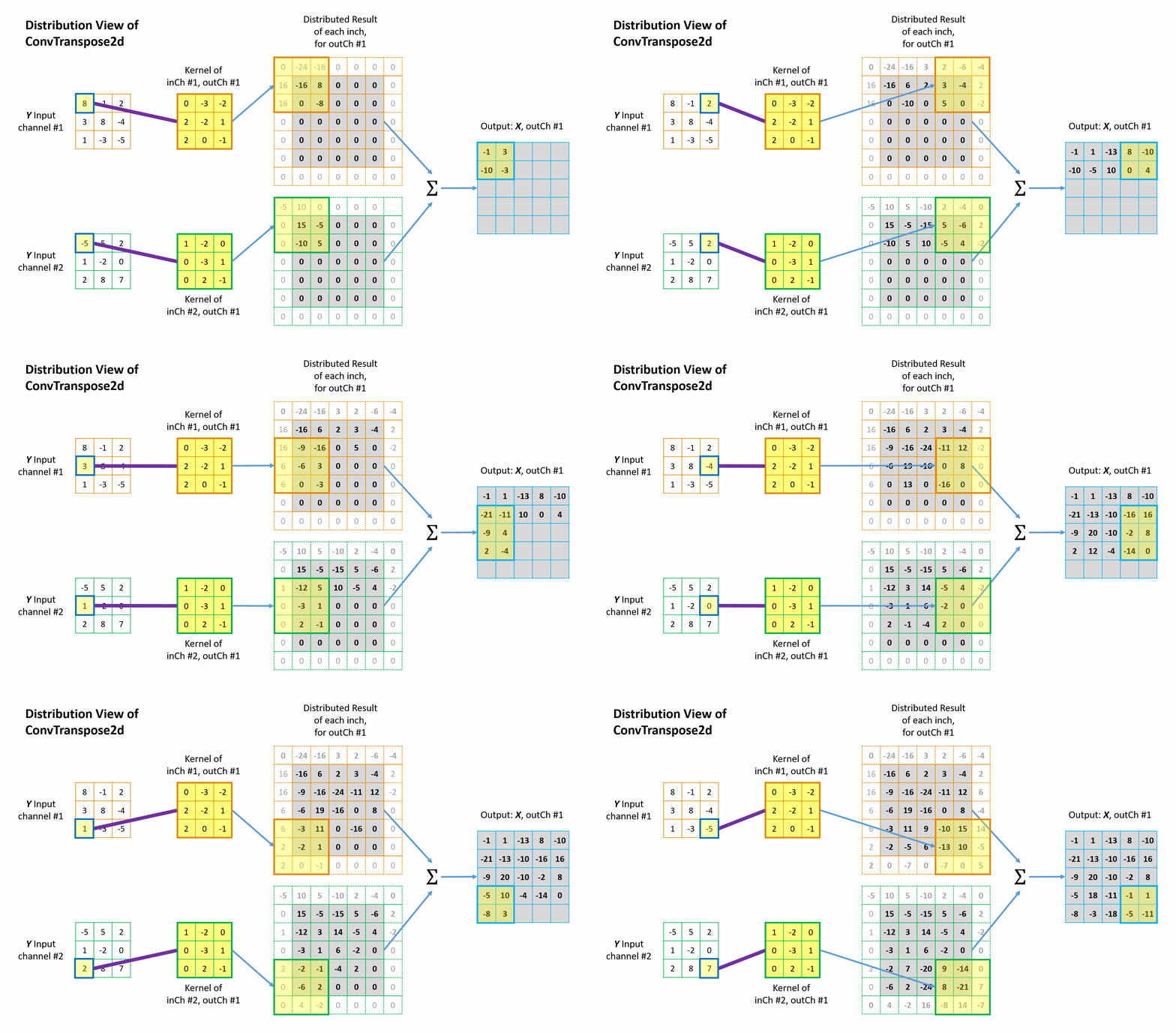
Figure 8 Animation of the mathematical operation of the transposed convolution from distrbution view.
The fundamental idea is quite simple: from the perspective view of the \({tc\_input}\) elements, “I will distribute my value back to whichever elements in the \(conv\_input\) contributed to me in the forward convolution process, with the weighting factors determined by the \(tc\_kernel\).” This is known as distribution view of transposed convolution. Straight-forward and fair.
2.2. Collection view of ConvTranspose2d
Equivalently, the mathematical operation of transposed convolution can also be explored from the perspective view of each element in the final \({tc\_output}\) matrices, known as collection view. In this view, transposed convolution is seen as another convolution, but with new and different inputs, kernels, padding and stride.
Still using the same example, the original forward convolution has input size \({N_{xIn\_conv}} = 5\), kernel size \({N_{v\_conv}} = 3\), padding \({P_{x\_conv}} = 1\), stride \({S_{x\_conv}} = 2\) in the horizontal direction, and the same for the vertical direction respectively and thus left out. Based on the equation from the previous post, its output size (which is also the input size for the transposed convolution) is
The parameters for the \(associated\) transposed convolution are
- New input size: the raw input size is \({N_{xIn\_tc}} = {N_{xOut\_conv}} = 3\) as above. However, because \({S_{x\_conv}} = 2\) was used in the forward convolution to reduce the matrix size, it is intuitive to expect to have a stride less than one (\( < 1.0\)) in the \(associated\) transposed convolution in order to increase the matrix size. This is called \(fractional stride\) and is equivalent to inserting \({S_{x\_conv}} - 1\) zeros between columns (and \({S_{y\_conv}} - 1\) zeros between rows). Therefore the new stretched input size is \({N_{xIn\_tc\_new} } = \left( { {N_{xIn\_tc} } - 1} \right) \times {S_{x\_conv}} + 1 = \left( {3 - 1} \right) \times 2 + 1 = 5\)
- Kernel size: kept the same as that in the forward convolution, \({N_{v\_tc}} = 3\). However, the new \(3 \times 3\) kernel of the transposed convolution need to be flipped in both horizontal and vertical directions.
- New padding: \({P_{x\_tc} } = {N_{v\_tc}} - 1 - {P_{ {x_{conv} } } } = 3 - 1 - 1 = 1\).
- New Stride: \({S_{x\_tc} } = 1\) and the fractional stride is realized by inserting \({S_{x/y\_conv} } - 1\) zeros between columns and rows.
In summary, the transposed convolution can be seen as a new convolution with \({N_{xIn\_tc\_new} } = 5\), \({N_{v\_tc} } = 3\), \({P_{x\_tc} } = 1\) and \({S_{x\_tc} } = 1\).
Figures 9 illustrates how the 1st element in the final \({tc\_output}\) is built up from the contribution of \(3 \times 3\)=9 elements in \({tc\_input}\) from the collection view of transposed convolution. The other elements are processed in the same way. Animation in Figure 10 illustrates the complete operations of this transposed convolution example. Please note a few things in the illustrations.
- Each element in \({tc\_output}\) collects contribution from a total of \(3 \times 3\)=9 elements of original \({tc\_input}\) via the \(3 \times 3\) tc_kernels. This 9-to-1 mapping pattern (including padding and stride) maintains the original 1-to-9 relationship in the forward convolution.
- The kernels are flipped in both horizontal and vertical directions.
- Zeros are inserted between rows and columns to equivalently achieve fractional stride and thus the matrix size is increased from \(3 \times 3\) to \(5 \times 5\) before padding at borders. The in the new convolution, the kernel slide only 1 step every time.
- All borders are padded with zeros using \({P_{x\_tc}} = 1\).
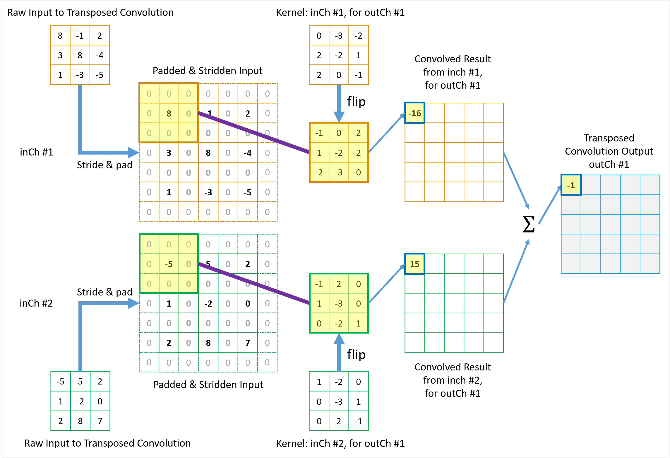
Figure 9 Illustration of how the 1st element in the \({tc\_output}\) is built up from \(3 \times 3\) elements in \({tc\_input}\) from collection view of transposed convolution.
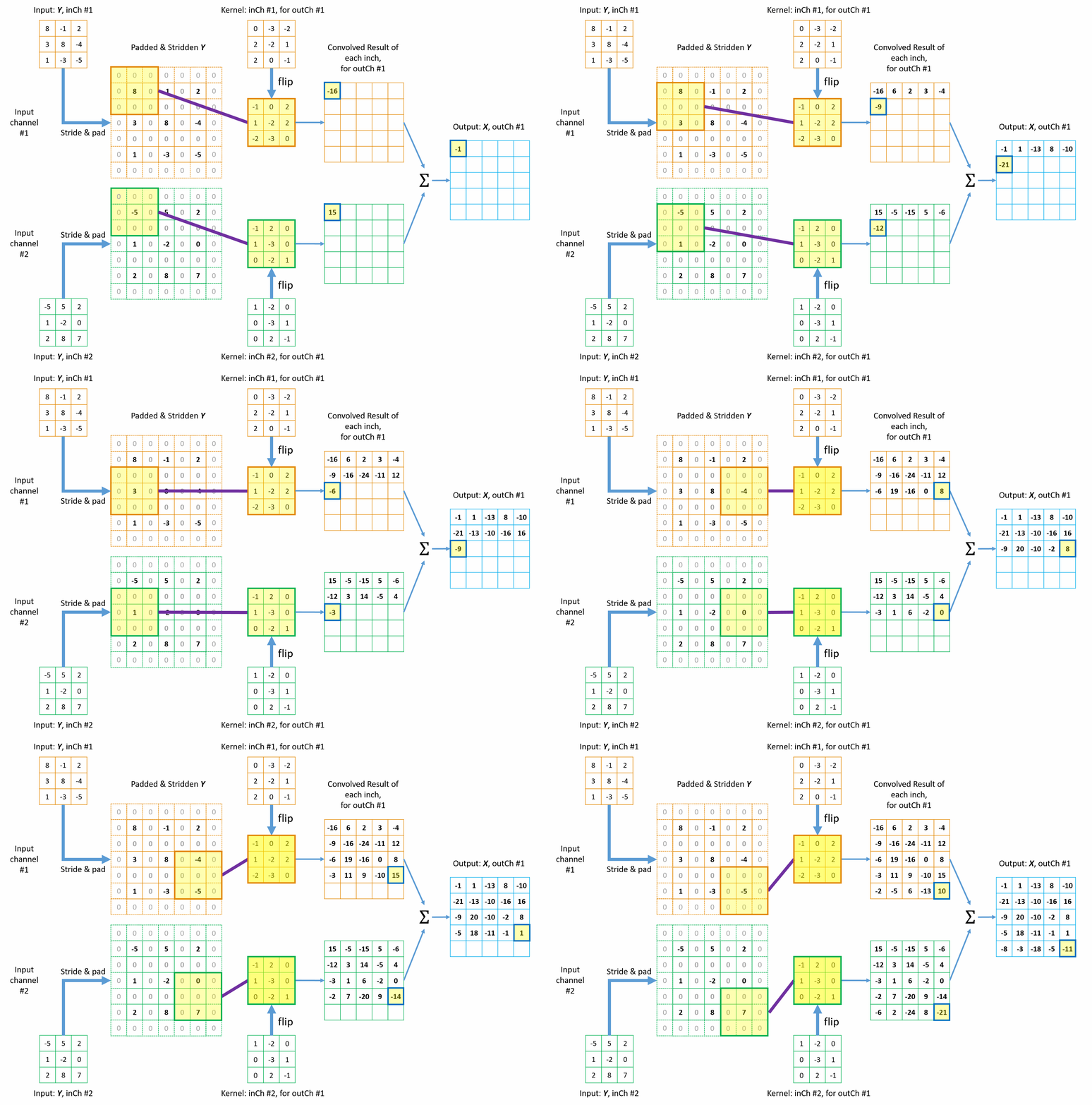
Figure 10 Animation of the mathmetical operation of the transposed convolution from collection view.
The fundamental idea is straight-forward too: from the perspective view of the \({tc\_output}\) elements, “I will collect my shares back from whichever elements in the \({conv\_output}\) (or \({tc\_input}\)) that I contributed to in the forward convolution process, with the weighting factors determined by the flipped tc_kernel.” This is known as collection view of transposed convolution.
3. Transposed Convolution Output Size
From the previous section, we have learnt the following relationship along the horizontal (\(x\)) direction for the transposed convolution as a new convolution:
\({N_{xIn\_tc\_new} } = \left( { {N_{xIn\_tc}} - 1} \right) \times {S_{x\_conv} } + 1\)
\({N_{v\_tc} } = {N_{v\_conv} } \equiv {N_v}\)
\({P_{x\_tc} } = {N_v} - 1 - {P_{x\_conv} }\)
\({S_{x\_tc} } = 1\)
(2)From the general equation for convolution output size we have
Substitute Equations (1) into Equation (2), we have
\({N_{xOut\_tc} } = \frac{ {\left( { {N_{xIn\_tc} } - 1} \right) \times {S_{x\_conv} } + 1 + 2\left( { {N_v} - 1 - {P_{x\_conv} } } \right) - {N_v} } } {1} + 1\)
\( = \left( { {N_{xIn\_tc} } - 1} \right) \times {S_{x\_conv} } + {N_v} - 2{P_{x\_conv} }\)
(4)Similarly, for the vertical direction, we have
In fact, Equations (3) and (4) matches the relationships given by PyTorch Documentation, where we assumed \(dilation\left[ {0\left] { = dilation} \right[1} \right] = 1\) (i.e. no dilation) in order to simplify the explanation.
Please also note that, due to the floor operation in the equation of the forward convolution output size \({N_{xIn\_tc} } \equiv {N_{xOut\_conv} } = \left\lfloor { \frac{ { {N_{xIn\_conv} } + 2{P_{x\_conv} } - {N_{v} } } } { { {S_{x\_conv} } } } } \right\rfloor + 1\), there are a total of \({S_{x\_conv}}\) different input sizes \({N_{xIn\_conv}}\) that can generate the same output size. Therefore, by default, transposed convolution maps back to the minimum size of \({N_{xIn\_conv}}\) that satisfies the relationship above. That’s why there is an argument parameter of “output_padding” in the transposed convolution modules, which controls the additional size added to one side of the output shape, default=0.
It is very important to point out that the argument parameters “stride” and “padding” defined the transposed convolution modules (e.g. \({ConvTranspose2d}\) [2]) are the stride and padding of the “forward” convolution, like \({S_{x\_conv}}\), \({S_{y\_conv}}\), \({P_{x\_conv}}\) and \({P_{y\_conv}}\) in this post, not the stride and padding of the associated transposed convolution.
4. The 1st Implementation of \({ ConvTranspose2d}\) (Forward and Backward)
In order to help gain hands-on experience and full understanding of transposed convolution, we implemented two versions of the \({ ConvTranspose2d}\). The 1st version is based on the distribution view and by subclassing \(torch\).\(autograd\).\(Function\) and manually overriding the forward and backward methods. The 2nd version is based on the collection view, which sees the transposed convolution as another convolution, and implemented as a function to use our custom implementations of \({ Conv2d }\) modules discussed in the previous post.
This section covers Version #1 and the compete source codes can be found on GitHub (my_convTranspose2d_v1_distrib_view.py).
4.1. Forward pass
The forward function is overridden to take 5 input arguments:
- ctx: represent THIS instance of the class
- Y: the 4-D tensor with a shape of (\({nImgSamples}\), \({ nInYCh }\), \({ nYRows }\), \({ nYCols }\)). This is input to the transposed convolution and also the output from the “original” forward convolution. In the previous post of convolution, variable \({ X }\) and \({ Y }\) are used as the input and output of the forward convolution, respectively. To be consistent with it, we used variables \({ Y }\) and \({ X }\) as the input and output of the “associated” transposed convolution here.
- in_weight: the 4-D learnable kernel of the transposed convolution with a shape of (\({ nInYCh }\), \({ nOutXCh }\), \({ nKnRows }\), \({ nKnCols }\)). Please note the change in the order of input and output channels.
- in_bias: 1-D learnable convolution bias with a shape of (\({ nOutXCh }\),)
- convparam: tuple to pass in parameters of (\(padding\), \(stride\)), default=(\(0,1\))
In the core part, a padded output matrix is allocated in the memory, which corresponds the 3rd column matrices in Figure 6, so that the distribution operation can be performed without worry about the border. The final output is extracted from the padded matrices to have a shape of (\({nImgSamples}\), \({ nOutXCh }\), \({ nOutXRows }\), \({ nOutXCols }\)) and then returned.
4.2. Backward pass
The backward function is overridden to take one argument (in addition to THIS instance ctx), which must match the output list of the forward function:
- ctx: represent THIS instance of the class
- grad_from_upstream: the 4-D tensor of the upstream gradient for the transposed convolution. It has the same shape as the forward output, (\({nImgSamples}\), \({ nOutXCh }\), \({ nOutXRows }\), \({ nOutXCols }\)).
The backward function must return the same number of items as the argument list of the forward function, not including ctx. More specifically, it must return 3 gradients of the loss w.r.t. to \({ Y }\), \({ in\_weight }\) and \({ in\_bias }\) (if specified, otherwise a \(None\)) respectively, plus a \(None\) for convparam that is just a tuple of parameters and does not require gradient.
Please see the source code for detailed implementation and it is quite self-explaining. In fact, it just applies the chain rule as discussed in the previous posts to compute gradients using 3-layers of nested loops in the same way as in the forward function.
5. The 2nd Implementation of ConvTranspose2d
The 2nd version of implementation is based on the collection view and treats \({ ConvTranspose2d}\) as a routine convolution with flipped kernels, new parameters of stride and padding, and the rearranged input matrices (with zeros inserted between rows and columns for fractional stride). To utilize our custom implementation of \({ Conv2d }\) from the last post, we simply define this version of \({ ConvTranspose2d}\) as a function instead of subclassing \(torch\).\(autograd\).\(Function\), and therefore there is no need to explicitly override the forward and backward functions. The interface of the function is
def MyConvTranspose2d_v2_Collect(Y, in_weight, in_bias=None, convparam=None)
where the arguments \({ Y }\), \({ in\_weight }\), \({ in\_bias }\) and \(convparam\) have the same definition as the 1st implementation.
Please see the complete source code of this implementation on GitHub (my_convTranspose2d_v2_collect_view.py). It’s self-explaining and straight-forward.
6. Validation against PyTorch Built-ins
Both implementations of transposed convolution are tested against the Torch built-in implementation. The test code can be found here. Results show that both implementations produced the same results as the Torch built-ins, including the output of transposed convolution and the gradients of loss w.r.t. the input, kernel and bias.
7. Summary
In this post, we discussed the fundamentals of transposed convolution for neural networks and demonstrated 2 different ways (distribution view and collection view) to implement it. While we just used \({ ConvTranspose2d}\) as the example, all ideas can be extended to \({ ConvTranspose1d}\) and \({ ConvTranspose3d}\). In next post, we will talk about various optimizers for neural networks.
8. References
- [1] Will Badr (2019) Auto-Encoder: What Is It? And What Is It Used For?
- [2] ConvTranspose2d - PyTorch documentation.