Understanding Artificial Neural Networks with Hands-on Experience - Part 5. Hyper-Parameter Learning Rate and Schedulers
This post is the 5th part of the series.
- Matrix Multiplication, Its Gradients and Custom Implementations
- Convolution, Its Gradients and Custom Implementations
- Transposed Convolution and Custom Implementations
- Optimization and optimizers with Custom Implementations and A Case Study
- Hyper-Parameter Learning Rate and Schedulers (this post)
In the previous post, we went through the fundamentals of optimization and discussed several widely used optimizers. In the neural network case study of ellipse semi-major axis and semi-minor axis regression task, there are several parameters (such as learning rate \(\alpha \), \({\beta _1}\), \({\beta _2}\), etc.) used in those optimizers to guide how aggressive or conservative to update the learnable parameters. To differentiate from learnable parameters, they are often called hyper-parameters. You may have already noticed from the example that different optimization algorithms used different learning rates and had different searching paths in the end. You may also wonder why not use the same learning rate in all scenariors for simplicity. We do have tried it, but it turned out there was no single learning rate that worked for all optimizers in this example, therefore, it need to be tuned up for individual optimizers. In fact, tune-up of hyper-parameters is important and necessary in most, if not all, deep learning applications. In this post, we will discuss one of the most important hyper-parameters, the learning rate, and the ways to help adapt it along with the training by using scheduler. For the convenience, this post is organized into the following sections.
- The same case study – but with revised implementation structure
- An important hyper-parameter: learning rate
- The same learning rate leading to different effective step size
- Impact of different learning rates and tune-up
- Adjusting learning rate with scheduler
- Summary
- References
1. The same case study – but with revised implementation structure
For demonstration purpose, we will use the same case study (regression of Earth-to-Mars transfer orbit) as used in the previous post. The regression task is, given \(N = 512\) pairs of the \(x\)- and \(y\)-coordinates sampled from the elliptical orbit with noise, to find the unknown parameters A and B in Equation (1).
The solution in this post is the same as that in the previous post. However, there are a few changes in the implementation.
First, in the previous post, the focus was to understand how optimization works in neural networks, so we included two implementations, one using Torch built-ins and the other one fully using custom code. In this post, the focus is the hyper-parameter, so we keep only the built-in version, but drop the custom version.
Second, in the previous post, the forward operations were explicitly coded line-by-line inside the mini-batch for loop. The purpose was to help digest what’s really going on underneath. In this post, the forward pass is wrapped into a module (named OrbitRegressionNet) that subclasses from the base class torch.nn.Module. Its constructor __init__(self, xaxisoffset, initWa, initWb) and the forward function forward(self, x) are overridden accordingly. This is a more standard practice in neural network applications. To use it, instantiate an object first:
thenet = OrbitRegressionNet(xaxisoffset, initWa, initWb)and then call it inside the mini-batch loop as follows
y_pred, negativeloc = thenet(x)where x is the mini-batch input samples.
Third, because of the change #2 above, the learnable parameters \(Wa\) and \(Wb\) must be declared as nn.Parameter object inside the constructor __init__(…) of the OrbitRegressionNet module.
self.Wa = nn.Parameter(initWa)self.Wb = nn.Parameter(initWb)Then they must be registered to the optimizer by calling thenet.parameters() as follows so that the optimizer knows they are the learnable parameters to be updated. Otherwise, Wa and Wb won’t be updated through the entire training process.
optimizer = optim.Adam(thenet.parameters(), lr=learning_rate, betas=(beta1, beta2), eps=eps)Fourth, instead of manually computing the MSE loss, an nn.MSELoss is declared
loss_fn = nn.MSELoss(reduction='mean')Then, the loss_fn is called inside the mini-batch loop as follows:
loss = loss_fn(y_pred[~negativeloc], y[~negativeloc])where \(y\_pred\) is the output from the network and \(y\) is the given truth.
Lastly, a few lines of log code is inserted between loss.backward() and optimizer.step() to record the status of the learnable parameters \(Wa\) and \(Wb\), as well as their gradients \(dWa\) and \(dWb\), respectively.
One example source code with these changes can be found here.
2. The learning rate hyper-parameter
Learning rate is (at least one of) the most important among all hyper-parameters. To evaluate its role in optimization, let’s revisit the 4 optimization algorithms briefly. For more details, please see the previous post. In this orbit regression example, the learnable parameters \({w_a}\) and \({w_b}\) can be treated as a vector \(\left( {\begin{array}{*{20}{c} }{ {w_a} }\\{ {w_b} }\end{array} } \right)\) and their update can be written as follows:
\(\left( {\begin{array}{*{20}{c} }{ {w_a}^{\left( {t + 1} \right)} }\\{ {w_b}^{\left( {t + 1} \right)} }\end{array} } \right) = \left( {\begin{array}{*{20}{c} }{ {w_a}^{\left( t \right)} }\\{ {w_b}^{\left( t \right)} }\end{array} } \right) - \alpha \cdot \left( {\begin{array}{*{20}{c} }{ {g_a}^{\left( t \right)} }\\{ {g_b}^{\left( t \right)} }\end{array} } \right)\) (2)
\(\left( {\begin{array}{*{20}{c} }{ {w_a}^{\left( {t + 1} \right)} }\\{ {w_b}^{\left( {t + 1} \right)} }\end{array} } \right) = \left( {\begin{array}{*{20}{c} }{ {w_a}^{\left( t \right)} }\\{ {w_b}^{\left( t \right)} }\end{array} } \right) - \alpha \cdot \left( {\begin{array}{*{20}{c} }{ {v_a}^{\left( t \right)} }\\{ {v_b}^{\left( t \right)} }\end{array} } \right)\) (3)
\(\left( {\begin{array}{*{20}{c} }{ {w_a}^{\left( {t + 1} \right)} }\\{ {w_b}^{\left( {t + 1} \right)} }\end{array} } \right) = \left( {\begin{array}{*{20}{c} }{ {w_a}^{\left( t \right)} }\\{ {w_b}^{\left( t \right)} }\end{array} } \right) - \alpha \cdot \left( {\begin{array}{*{20}{c} }{\frac{ { {g_a}^{\left( t \right)} } }{ {\sqrt { {s_a}^{\left( t \right)} } } } }\\{\frac{ { {g_b}^{\left( t \right)} } }{ {\sqrt { {s_b}^{\left( t \right)} } } } }\end{array} } \right)\) (4)
\(\left( {\begin{array}{*{20}{c} }{ {w_a}^{\left( {t + 1} \right)} }\\{ {w_b}^{\left( {t + 1} \right)} }\end{array} } \right) = \left( {\begin{array}{*{20}{c} }{ {w_a}^{\left( t \right)} }\\{ {w_b}^{\left( t \right)} }\end{array} } \right) - \alpha \cdot \left( {\begin{array}{*{20}{c} }{\frac{ { {v_a}^{\left( t \right)} } }{ {\sqrt { {s_a}^{\left( t \right)} } } } }\\{\frac{ { {v_b}^{\left( t \right)} } }{ {\sqrt { {s_b}^{\left( t \right)} } } } }\end{array} } \right)\) (5)
Equations (2)-(5) represent the algorithms of SGD, SGD with momentum, RMSprop and Adam algorithms, respectively. In these equations, \(t\) denotes the number of updates, \(\left( {\begin{array}{*{20}{c} }{ {g_a} }\\{ {g_b} }\end{array} } \right)\) is the gradient of the loss w.r.t. \(\left( {\begin{array}{*{20}{c} }{ {w_a} }\\{ {w_b} }\end{array} } \right)\), \(\left( {\begin{array}{*{20}{c} }{ {v_a} }\\{ {v_b} }\end{array} } \right)\) is the exponentially weighted average of the gradient, \(\left( {\begin{array}{*{20}{c} }{ {s_a} }\\{ {s_b} }\end{array} } \right)\) is the exponentially weighted average of the squared gradient. \(\left( {\begin{array}{*{20}{c} }{\frac{ { {g_a}^{\left( t \right)} } }{ {\sqrt { {s_a}^{\left( t \right)} } } } }\\{\frac{ { {g_b}^{\left( t \right)} } }{ {\sqrt { {s_b}^{\left( t \right)} } } } }\end{array} } \right)\) and \(\left( {\begin{array}{*{20}{c} }{\frac{ { {v_a}^{\left( t \right)} } }{ {\sqrt { {s_a}^{\left( t \right)} } } } }\\{\frac{ { {v_b}^{\left( t \right)} } }{ {\sqrt { {s_b}^{\left( t \right)} } } } }\end{array} } \right)\) can be thought of as the adjusted gradient and momentum, respectively, as adjusted by a scaling factor of \(\left( {\begin{array}{*{20}{c} }{\frac{1}{ {\sqrt { {s_a}^{\left( t \right)} } } } }\\{\frac{1}{ {\sqrt { {s_b}^{\left( t \right)} } } } }\end{array} } \right)\).
The terms in \(\left( {\begin{array}{*{20}{c} }{}\\{}\end{array} } \right)\) represent vectors in the \({w_a}\)-\({w_b}\) 2D space. So they can be rewritten as a product of the magnitude and unit vector, and Equation (2)-(5) can be rewritten as
\(\left( {\begin{array}{*{20}{c} }{ {w_a}^{\left( {t + 1} \right)} }\\{ {w_b}^{\left( {t + 1} \right)} }\end{array} } \right) = \left( {\begin{array}{*{20}{c} }{ {w_a}^{\left( t \right)} }\\{ {w_b}^{\left( t \right)} }\end{array} } \right) - \left( {\alpha \sqrt { {g_a}{ {^{\left( t \right)} }^2} + {g_b}{ {^{\left( t \right)} }^2} } } \right) \cdot \left( {\begin{array}{*{20}{c} }{ {u_{a,SGD} }^{\left( t \right)} }\\{ {u_{b,SGD} }^{\left( t \right)} }\end{array} } \right)\) (6)
\(\left( {\begin{array}{*{20}{c} }{ {w_a}^{\left( {t + 1} \right)} }\\{ {w_b}^{\left( {t + 1} \right)} }\end{array} } \right) = \left( {\begin{array}{*{20}{c} }{ {w_a}^{\left( t \right)} }\\{ {w_b}^{\left( t \right)} }\end{array} } \right) - \left( {\alpha \sqrt { {v_a}{ {^{\left( t \right)} }^2} + {v_b}{ {^{\left( t \right)} }^2} } } \right) \cdot \left( {\begin{array}{*{20}{c} }{ {u_{a,Momentum} }^{\left( t \right)} }\\{ {u_{b,Momentum} }^{\left( t \right)} }\end{array} } \right)\) (7)
\(\left( {\begin{array}{*{20}{c} }{ {w_a}^{\left( {t + 1} \right)} }\\{ {w_b}^{\left( {t + 1} \right)} }\end{array} } \right) = \left( {\begin{array}{*{20}{c} }{ {w_a}^{\left( t \right)} }\\{ {w_b}^{\left( t \right)} }\end{array} } \right) - \left( {\alpha \sqrt {\frac{ { {g_a}{ {^{\left( t \right)} }^2} } }{ { {s_a}^{\left( t \right)} } } + \frac{ { {g_b}{ {^{\left( t \right)} }^2} } }{ { {s_b}^{\left( t \right)} } } } } \right) \cdot \left( {\begin{array}{*{20}{c} }{ {u_{a,RMSprop} }^{\left( t \right)} }\\{ {u_{b,RMSprop} }^{\left( t \right)} }\end{array} } \right)\) (8)
\(\left( {\begin{array}{*{20}{c} }{ {w_a}^{\left( {t + 1} \right)} }\\{ {w_b}^{\left( {t + 1} \right)} }\end{array} } \right) = \left( {\begin{array}{*{20}{c} }{ {w_a}^{\left( t \right)} }\\{ {w_b}^{\left( t \right)} }\end{array} } \right) - \left( {\alpha \sqrt {\frac{ { {v_a}{ {^{\left( t \right)} }^2} } }{ { {s_a}^{\left( t \right)} } } + \frac{ { {v_b}{ {^{\left( t \right)} }^2} } }{ { {s_b}^{\left( t \right)} } } } } \right) \cdot \left( {\begin{array}{*{20}{c} }{ {u_{a,Adam} }^{\left( t \right)} }\\{ {u_{b,Adam} }^{\left( t \right)} }\end{array} } \right)\) (9)
Now the physics meaning of these equations becomes more clear. The unit vectors \(\left( {\begin{array}{*{20}{c} }{ {u_{a,SGD} }^{\left( t \right)} }\\{ {u_{b,SGD} }^{\left( t \right)} }\end{array} } \right)\), \(\left( {\begin{array}{*{20}{c} }{ {u_{a,Momentum} }^{\left( t \right)} }\\{ {u_{b,Momentum} }^{\left( t \right)} }\end{array} } \right)\), \(\left( {\begin{array}{*{20}{c} }{ {u_{a,RMSprop} }^{\left( t \right)} }\\{ {u_{b,RMSprop} }^{\left( t \right)} }\end{array} } \right)\) and \(\left( {\begin{array}{*{20}{c} }{ {u_{a,Adam} }^{\left( t \right)} }\\{ {u_{b,Adam} }^{\left( t \right)} }\end{array} } \right)\) represent the directions of the gradients or momentums, whereas the combined magnitude terms \(\alpha \sqrt { {g_a}{ {^{\left( t \right)} }^2} + {g_b}{ {^{\left( t \right)} }^2} } \), \(\alpha \sqrt { {v_a}{ {^{\left( t \right)} }^2} + {v_b}{ {^{\left( t \right)} }^2} } \), \(\alpha \sqrt {\frac{ { {g_a}{ {^{\left( t \right)} }^2} } }{ { {s_a}^{\left( t \right)} } } + \frac{ { {g_b}{ {^{\left( t \right)} }^2} } }{ { {s_b}^{\left( t \right)} } } } \) and \(\alpha \sqrt {\frac{ { {v_a}{ {^{\left( t \right)} }^2} } }{ { {s_a}^{\left( t \right)} } } + \frac{ { {v_b}{ {^{\left( t \right)} }^2} } }{ { {s_b}^{\left( t \right)} } } } \) represent the actual update step size, and the ‘\( - \)’ indicates the opposite directions of the unit vectors.
2.1. The same learning rate leading to different effective step size
The performance of training heavily depends on effective step size, which in turn depends on the learning rate as well. In the first investigation, we will take a look at how the actual (effective) step size varies through the training process and varies for different optimizers when the same learning rate \(\alpha \) is used. To demonstrate the impact, we choose \(\alpha = 0.01\) for all of the 4 optimizers and keep it unchanged through the whole process of training. Please note that, \(\alpha = 0.01\) definitely is not optimal for some optimizers (for example, Adam), the same value was used here just for comparison purpose.
Because the Torch built-in optimizers don’t provide information of the intermediate variables during training, such as gradient \(g\), momentum \(v\), weighted average of squared gradient \(s\), unit vectors, step size, etc., we continue to use some scripts from the previous post (SGD, SGD_momentum, RMSprop and Adam) with modifications to record the histories of those intermediate variables. You can find the log files here (SGD_log, Momentum_log, RMSprop_log and Adam_log) or you can also use the Python scripts to generate those files. The Python script to parse those data and generate the figures/videos can be found here.
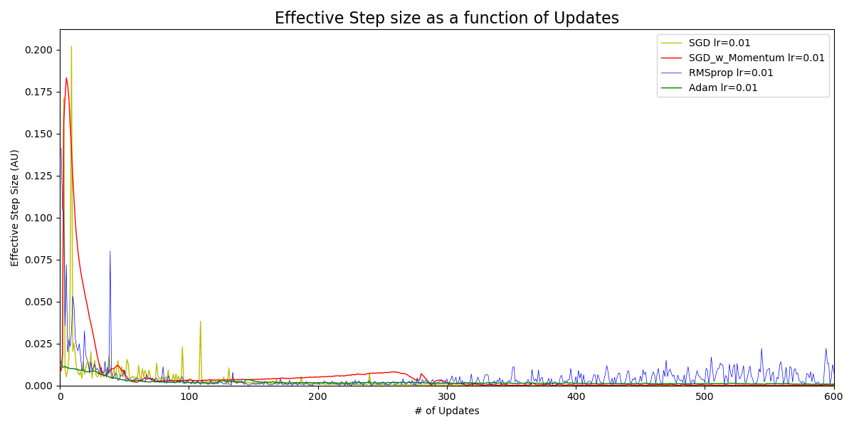
Figure 1 The effective step size vs the number of updates through training, for the same learning rate.
Figure 1 show the plots of the effective step size as a function of the number of updates. A few things can be observed.
- While the learning rate is the same, the effective step size varies for these optimizers. In this specific example, the effective step size of Adam (the green curve) is much smaller but also smoother than the others, especially during the earlier stages. This means that it tends to converge relatively slower. It could also suggest that a greater value of learning rate can be more optimal. In fact, it is.
- The effective step size also varies for individual optimizers. This is because the gradients of Wa and Wb are different at different location, so are the momentum and the squared gradients, and, in turn, so is the effective step size.
- For the red curve (SGD with momentum), the effective step size decreases first, and then increases consistently from about \(70\) updates through \(270\) updates. This might suggest there is some special behavior there during the training. In fact, it does bypass the target and then turns around to come back, as we will show it in animations later.
- Different from the other curves, there is relatively big fluctuation in the blue curve (RMSprop) starting from \(300\) updates. This might suggest that the learning rate is too big, thus the effective step size is also too big so that the training keeps dancing around the target location instead of converging to it. A better strategy is to reduce the learning rate, which in turn reduces the effective step size to avoid over-step.
Figure 2 shows the first four steps of updates using these optimizers. Each arrow represents one step and the length indicates its effective step size. All of them start from the same point of (\(Wa = 0.1\) and \(Wb = 1.8\)) in the 2D contour plot. However, due to variation of the gradients in the 2D space and the different algorithms, the four optimizers quickly take different paths and different converge speed. If you would like to know how each step is determined exactly, you can check the intermediate variables recorded in the log files.
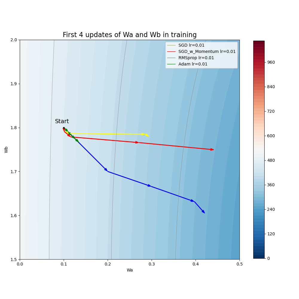
Figure 2 Illustration of the first four steps during the training.
Animation of how the 4 optimizers search the path from the starting point to the target point (corresponding to the minimum loss) is illustrated in Figure 3. We can see from the animation that the green curve (Adam) is slower from the beginning than the others, matching the observation in the 1st bullet above. The red curve (SGD with momentum) does overshoot and bypass the target and then has to turn around, also matching the 3rd bullet above. The purple curve (RMSprop) does keep jumping around the target point after it approaches the minimum loss point, which matches the 4th bullet discussion above.
Figure 3 Animation of the four optimizers’ update paths from the starting point to the minimum loss.
Based on this experiment, we know that there is no universal optimal learning rate that works for all optimizers. In fact, different optimization algorithms have different optimal learning rates. So tune-up of the learning rate is necessary and important.
The source code used in this section can be found on GitHub for SGD, SGD with Momentum, RMSprop, Adam and data plot & animation. The corresponding raw data and results can be found here.
2.2. Impact of different learning rates and tune-up
In this experiment we use the SGD_momentum optimizer as an example to investigate the impact of using different learning rates on training. A total of \(5\) learning rates are tested, including (from greatest to smallest) \(0.012\), \(0.01\), \(0.005\), \(0.001\) and \(0.00015\). In each test case, the learning rate remains unchanged through the process of training. \(Epoch = 100\) is used these test cases. Figures (4) through (8) show the regression results coming out from the training using these learning rates.
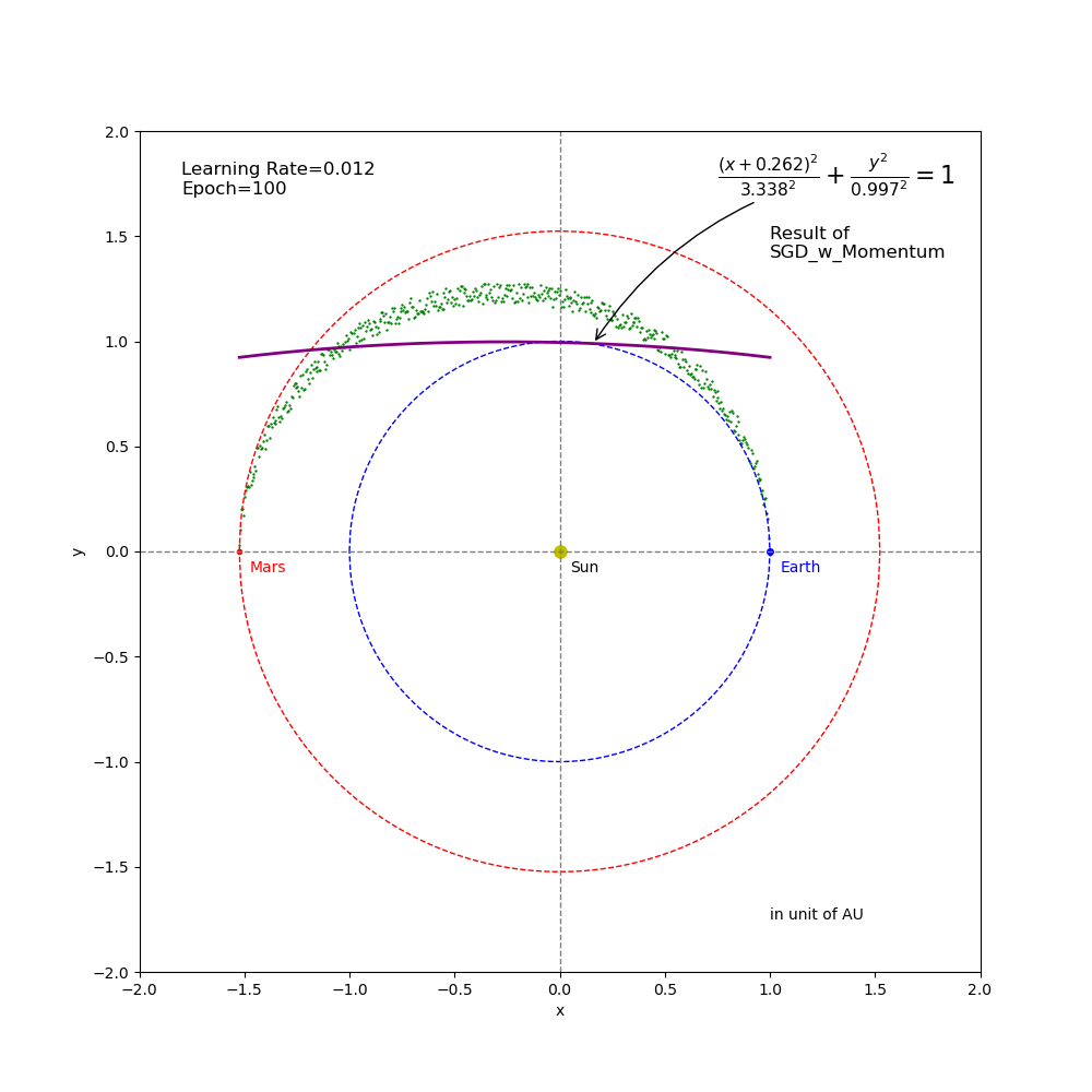
Figure 4 Regression result from SGD_Momentum training (epoch=100 and learning rate=0.012).

Figure 5 Regression result from SGD_Momentum training (epoch=100 and learning rate=0.01).

Figure 6 Regression result from SGD_Momentum training (epoch=100 and learning rate=0.005).
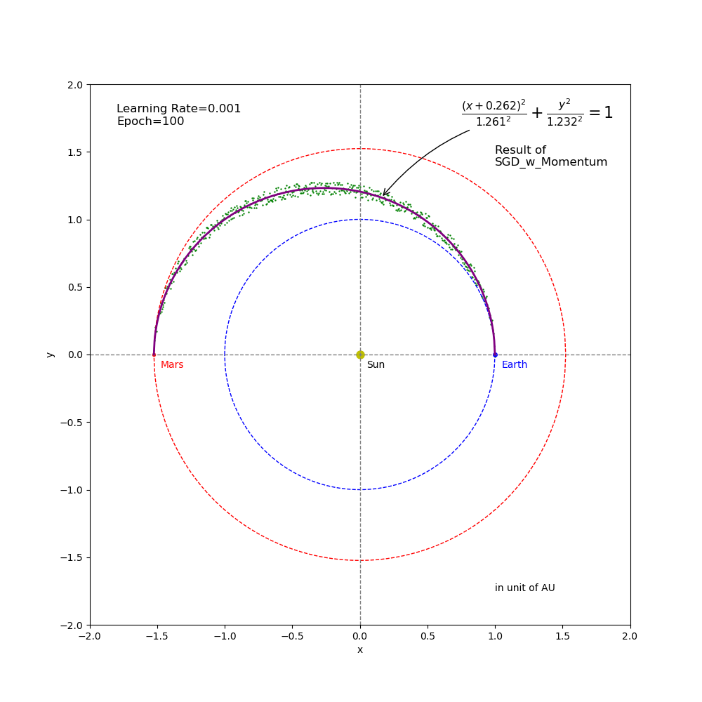
Figure 7 Regression result from SGD_Momentum training (epoch=100 and learning rate=0.001).
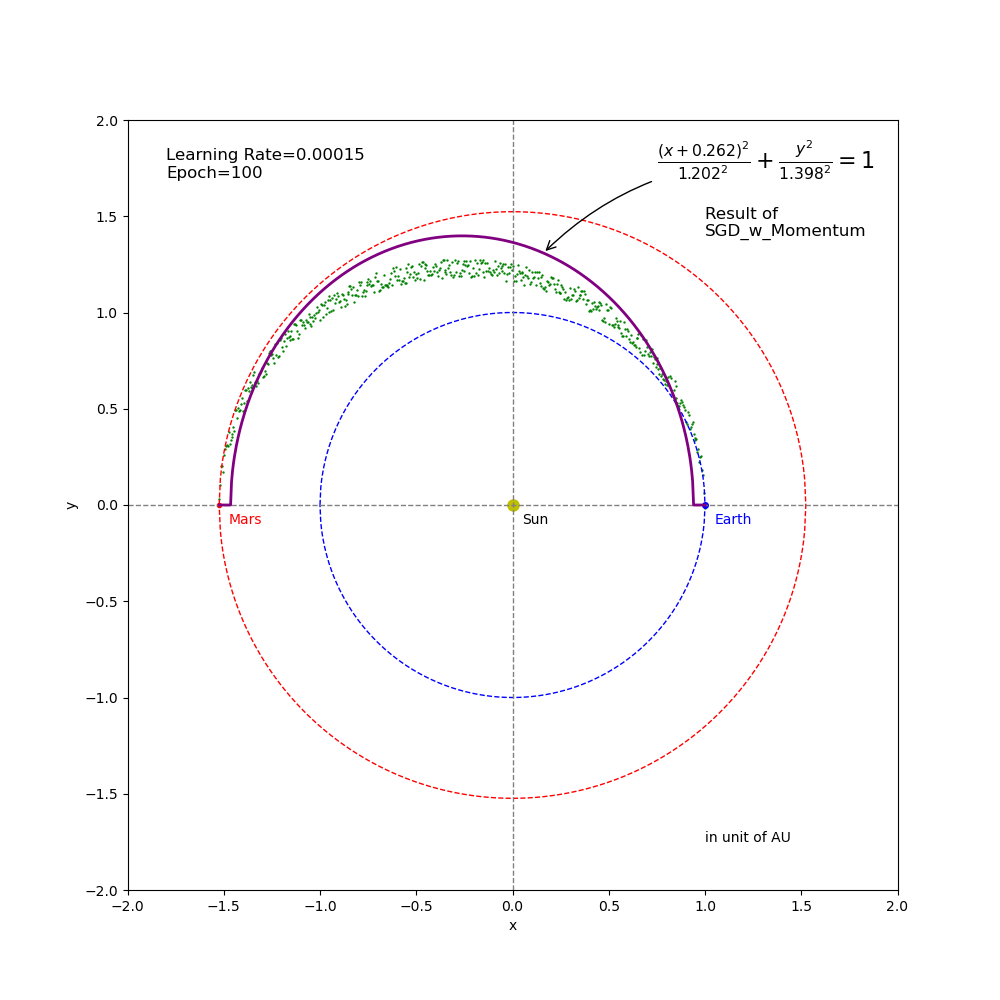
Figure 8 Regression result from SGD_Momentum training (epoch=100 and learning rate=0.00015).
A few things can be observed from these figures.
- The result of \(learningRate = 0.012\) (Figure 4) is far away from the ground truth in both the predicted orbit shape and the learnable parameters of \(Wa\) (\(3.338\) vs \(1.261\)) and \(Wb\) (\(0.997\) vs \(1.233\)). This was caused by two factors: (1) the fixed learning rate was too big and, with the momentum, the training path bypassed the target point; and (2) the number of epochs is only \(100\) so that the training ended before it could be fully corrected.
- The learning rates of \(0.01\) (Figure 5), \(0.005\) (Figure 6) and \(0.001\) (Figure 7) got fully converged to the target point through the \(100\) epochs of training. However, they have different paths and converge speeds. Among these 3 settings, \(0.01\) is the best candidate for learning rate in this specific example.
- The learning rate of \(0.00015\) (Figure 8) is another extreme opposite to the learning rate of \(0.012\). It is too small and thus the path searching speed is so slow that it couldn’t reach the target point before the end of training.
Animation of the path searching processes is illustrated in Figure 9, which also tells the stories about the Figures above.
Figure 9 Animation of the four optimizers’ update paths from the starting point to the minimum loss using different learning rates.
For the two failed test cases (using the learning rate of \(0.012\) that is too big and \(0.00015\) that is too small), we would like to see whether more epochs help or not. Therefore, we increased the number of epochs from \(100\) to \(400\). The results (Figures 10 and 11 below) show that it did help. Animation in Figure 12 illustrates how the additional epochs help the training continue to converge.
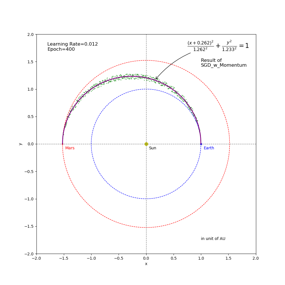
Figure 10 Regression result from SGD_Momentum training (epoch=400 and learning rate=0.012).
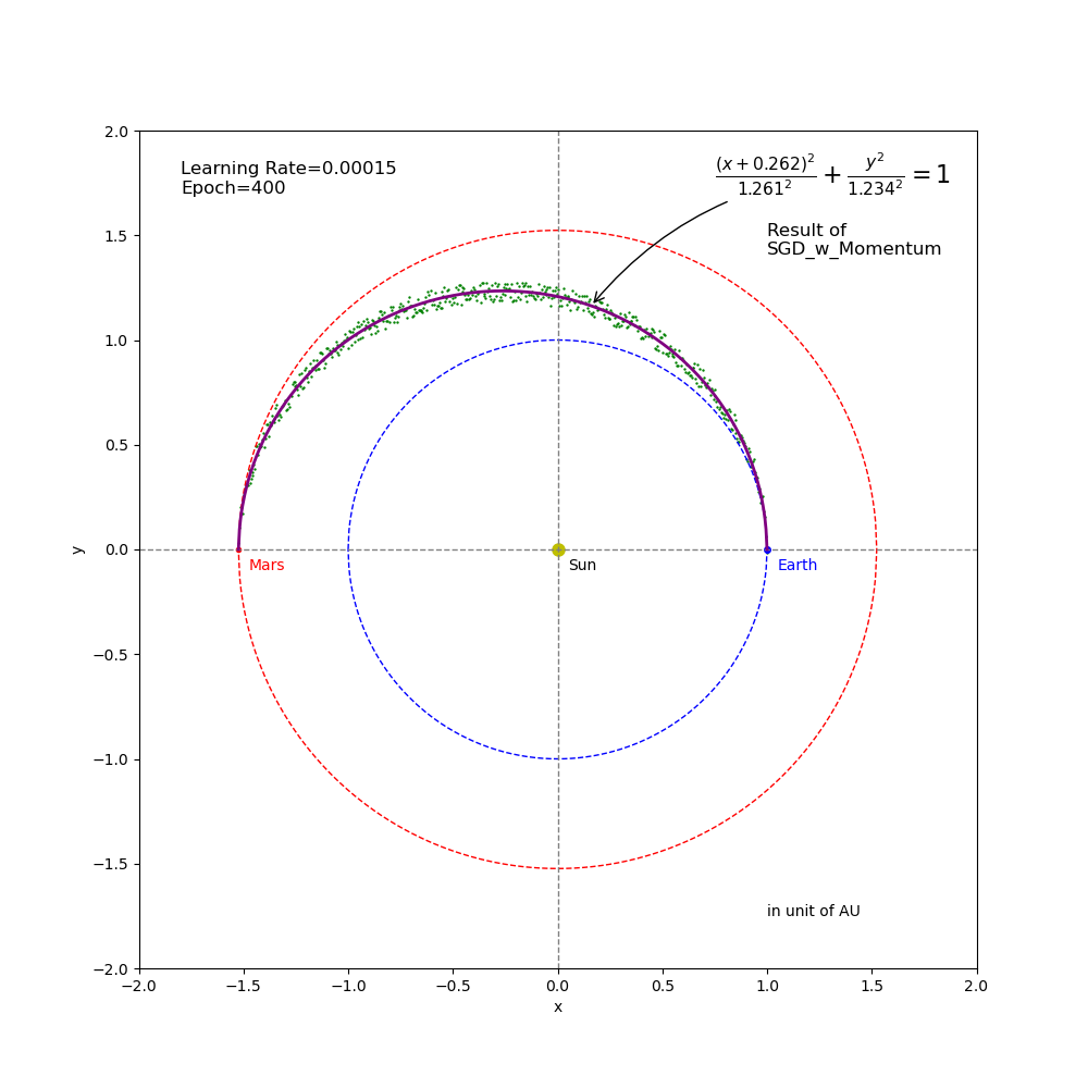
Figure 11 Regression result from SGD_Momentum training (epoch=400 and learning rate=0.00015).
Figure 12 Animation of the SGD-Momentum training paths to converge with additional epochs.
BTW, if you pay attention to the training path of \(learning\;rate = 0.012\) after it turns around towards left, you can see how amazing the momentum algorithm helps dampen oscillations in the vertical (\(Wb\)) direction and stay in the horizontal (\(Wa\)) direction. In fact, as shown in Figure 13, the gradient of \(Wb\) oscillates much more dramatically than the gradient of \(Wa\). Therefore, if the standard SGD algorithm is used without momentum, the training path will also oscillate back and forward in the \(Wb\) direction much more dramatically too.
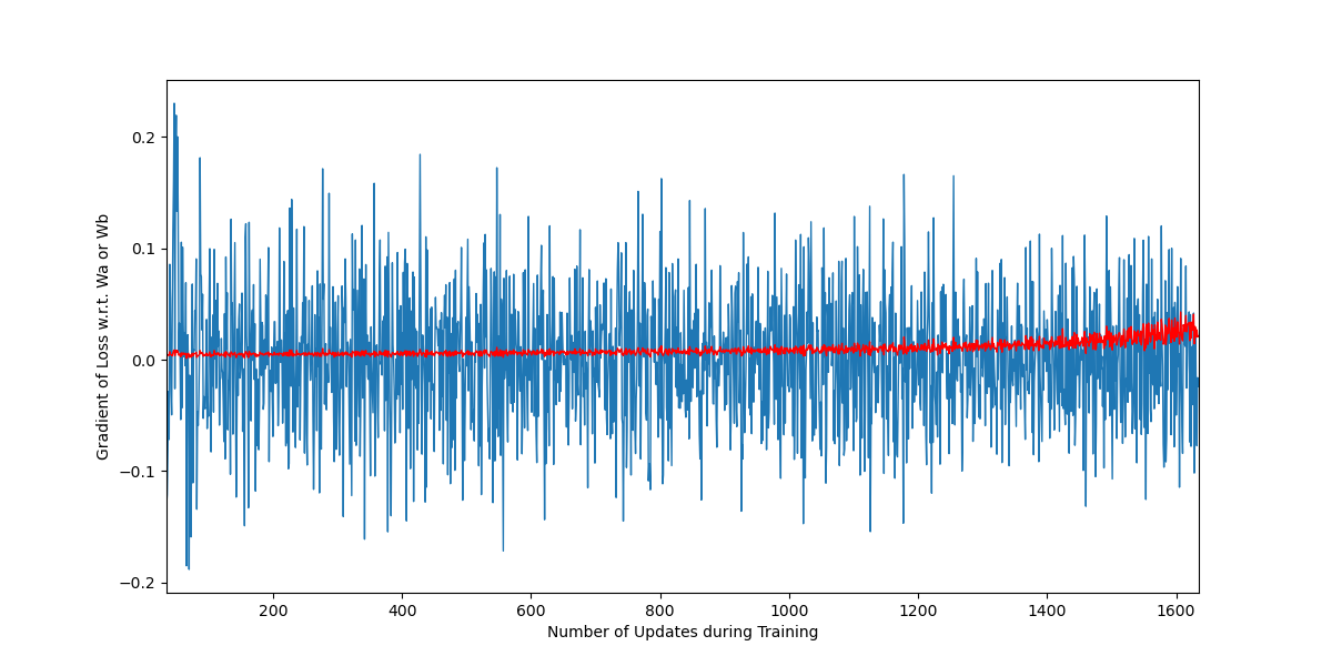
Figure 13 Gradient of Wa and Wb during the training in the left-ward segment (SGD_Momentum with epochs=400 and learning rate=0.012), which corresponds to updates from 35th to 1635th.
In this section, we used the optimizer of SGD with momentum as an example to demonstrate how the fixed learning rate impacts the training process. The ideas applied here can also be extended to other optimizers. The key message to take is that the hyper-parameter of learning rate plays an important role in training and performance of neural networks. The optimal value of learning rate is typically task-dependent and, in general, requires tune-up.
The source code used in this section can be found on GitHub for SGD with Momentum, data plot & animation with the same epochs , and data plot & animation with the extra epochs . The corresponding raw data and results can be found here.
3. Adjusting learning rate with scheduler
So far, we have been using fixed learning rates in the experiments. An obvious drawback of fixed learning rates is that, if learning rate is small, the effective step size will be small too, and thus the training will be slow. On the other hand, if learning rate is too big, the effective step size will be big and could lead to oscillation around the target point. An intuitive solution is to make learning rate adaptive or adjustable – relatively bigger at earlier stages of training and smaller at later stages. This feature can be realized with learning rate schedulers, which is supported in most platforms, such as PyTorch and Tensorflow. While there are different adjustment strategies, here we will discuss just some basic schedulers to gain the concepts of how schedulers work in neural networks. You can easily explore a variety of fancy schedulers for your projects, if needed. Again, we will continue to use the Orbit regression case study as an example to demonstrate how to use Torch built-in schedulers in the torch.optim.lr_scheduler package to control learning rate.
3.1. How to use scheduler?
In PyTorch, a scheduler object always takes an optimizer as well as some optional parameters as the input arguments for its constructor. The object should be instantiated before the training loop and be applied after the optimizer’s update inside the loop. The following code shows an example that uses MultiStepLR scheduler. Other types of schedulers can be used in a similar way, but may require different arguments.
lr_milestones = [4, 8, 10, 12, 14, 16, 18]
lr_gamma = 0.8
scheduler = torch.optim.lr_scheduler.MultiStepLR(optimizer, milestones=lr_milestones, gamma=lr_gamma)

for t in range(epoch):
    for i_batch, sample_batched in enumerate(xy_dataloader):
	…
	loss.backward()
	optimizer.step()
	scheduler.step()
3.2. The MultiStepLR scheduler
MultiStepLR scheduler decays the learning rate in the optimizer by a multiplicative factor (named gamma) once the number of updates (please note: not epochs) reaches the milestones in a pre-defined list. The factor gamma, \(\gamma \), should be between \(0\) and \(1\) so that the learning rate decreases. Mathematically, the adjustment of learning rate \(\alpha \) at \(t\)-th can be written as
In this experiment, we tested the following configurations:
Case 1: \(\alpha = 0.01\), fixed
Case 2: \(\alpha = 0.12\), fixed
Case 3: initial \(\alpha = 0.12\), MultiStepLR with \(\gamma = 0.80\), milestones=[4, 8, 10, 12, 14, 16, 18, 20, 22, 24]
Case 4: initial \(\alpha = 0.12\), MultiStepLR with \(\gamma = 0.50\), milestones=[5, 10, 15, 20]
Animation in Figure 14 illustrates how the MultiStepLR scheduler helped converge fast while avoiding over-shooting. The changes in the learning rate can be monitored by accessing optimizer.param_groups[0]['lr']. Figure 15 shows the decay of the learning rates due to the use of the schedulers for first 30 updates in Case 3 and Case 4, respectively. The source code used in this section can be found on GitHub for data generation using Adam optimization, and plot & animation . The corresponding raw data and results can be found here.
Figure 14 Animation of the training paths using Adam optimizer with and without the MultiStepLR schedulers.
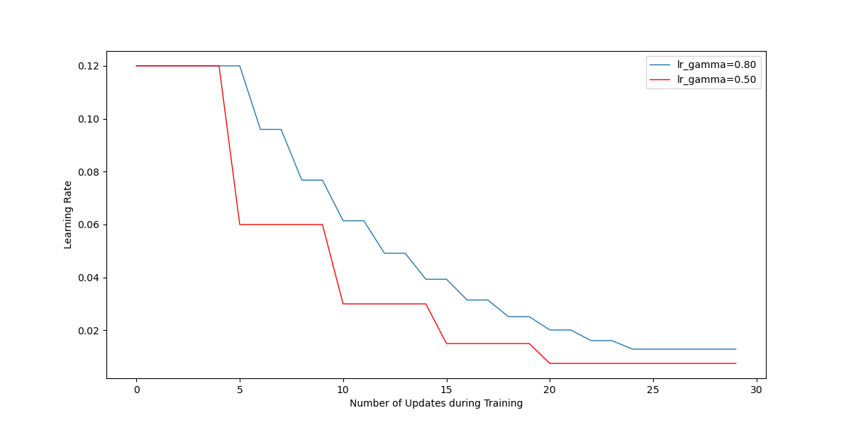
Figure 15 Adjustment of the learning rates during training by using schedulers.
3.3. The MultiplicativeLR scheduler
MultiplicativeLR is another scheduler to decay learning rate by a multiplicative factor that is computed from a specified lambda function. The lambda function provides a much more flexibility and can be customized based on the needs. It takes an integer argument that represents the count of updates performed so far. Mathematically, the adjustment of learning rate \(\alpha \) can be written as
where \(t\) denotes the count of updates.
In this experiment, we tested the following configurations:
Case 1: \(\alpha = 0.01\), fixed
Case 2: \(\alpha = 0.12\), fixed
Case 3: initial \(\alpha = 0.12\), using MultiplicativeLR with a lambda function that adjusts the learning rate by a factor of \(0.80\) at the following updates \(6, 8, 10, 12, 14, 16, 18, 20, 22\) and \(24\)
Case 4: initial \(\alpha = 0.12\), using MultiplicativeLR with a lambda function that adjusts the learning rate by a factor of \(0.50\) at the following updates \(5, 10, 15\) and \(20\)
These cases are very similar to those in the previous section, but we will use the MultiplicativeLR scheduler with lambda function instead. The code to instantiate the MultiplicativeLR scheduler looks like
lambda0_8 = lambda epoch: 0.8 if (epoch >= 6 and epoch <= 24 and epoch % 2 == 0) else 1.0
scheduler = torch.optim.lr_scheduler.MultiplicativeLR(optimizer, lr_lambda=lambda0_8)

# lambda0_5 = lambda epoch: 0.5 if (epoch >= 5 and epoch <= 20 and epoch % 5 == 0) else 1.0
# scheduler = torch.optim.lr_scheduler.MultiplicativeLR(optimizer, lr_lambda=lambda0_5)
The results are illustrated in Figure 16. We can also check the changes of learning rate in the log file. The source code used in this section can be found on GitHub for data generation using Adam optimization, and plot & animation . The corresponding raw data and results can be found here
Figure 16 Animation of the training paths using Adam optimizer with and without the MultiplicativeLR schedulers.
4. Summary
In this post, we used the elliptical orbit regression case study to demonstrate two things in neural networks: 1) impact of learning rate, which is one of the most important hyper-parameters of optimization algorithms, on training convergence and the importance of its tune-up case by case; and 2) how to use schedulers to adjust learning rate for better convergence and performance. There are other optimizers and learning rate schedulers available that is not covered in this post, but the basic ideas and experiences discussed here can be applied to those optimizers and schedulers as well.