Understanding Artificial Neural Networks with Hands-on Experience - Part 2. Convolution, Its Gradients and Custom Implementations
In the previous post, we discussed matrix multiplication and derivation of its gradients. In this post, we will talk about convolution, the 2nd part of the series.
- Matrix Multiplication, Its Gradients and Custom Implementations
- Convolution, Its Gradients and Custom Implementations (this post)
- Transposed Convolution and Custom Implementations
- Optimization and optimizers with Custom Implementations and A Case Study
- Hyper-Parameter Learning Rate and Schedulers
Because 2-dimensional (2-D) scenarios are the most common one in image deep learning, we will use 2-D convolution, referred to as Conv2d, as an example through this post, but the fundamentals can be extended to 1-D and 3-D scenarios as well. Please note that the two dimensions above means the height and width of an image. The other dimensions, such as batch samples and feature channels of each sample, are not counted here. Therefore, if the batch sample and feature channel dimensions are also considered, a batch of 2-D data will be represented in a 4-D tensor [Samples, Channels, Height, Width]: the 1st dimension for the batch samples, the 2nd one for feature channels, the 3rd one for height, and the 4th one for width. However, the basic convolution operations (including padding, stride, etc.) are performed within the height-width plane, not across the feature channels or batch samples. This is why it is called 2-D convolution even though 4-D tensors are actually used. Similarly, batch data in 1-D and 3-D scenarios will be represented in 3-D and 5-D tensors, respectively, but the corresponding convolution is still called 1-D convolution and 3-D convolution, respectively.
Hands-on practice is the best teacher for learning, so we will also demonstrate how to implement our own versions of Conv2d, including both forward and backward propagation. By going through this example, we hope it helps gain clear understanding of the concepts of Conv2d, output image dimensions, and how to calculate its gradients of weights, bias and inputs. Here are the outlines of this post.
- Conv2d
- Input and output dimensions
- Implementation #1 of Conv2d forward and backward
- Implementation #2 of Conv2d forward and backward
- Validation against the Torch Build-ins
- Summary
- Extra - Edge detector and smoothing using Conv2d
- References
1. Conv2d
Discrete convolution is used in neural networks to extract features of input images by applying a dot product with a sliding kernel. Let’s introduce two terminologies relevant to convolution:
- Stride: the step size (in unit of pixels) of the kernel when sliding over the input image. When the step size is 1 (stride=1), it is called unit stride.
- Padding: Padding means to extend the input image area by adding extra columns and rows of pixels to the outside border of the image. If all added pixels are filled with value zero, it is called zero-padding, which is the most common mode of padding.
1.1. Basic Conv2d with unit stride and no padding
We will start with the simplest case: Stride=1 and no padding. Given an input image \(\boldsymbol {I}\left( {y,x} \right)\) with an image size of \(\left( { {N_y},{N_x} } \right)\) and a sliding kernel \( \boldsymbol {K} \left( {u,v} \right)\) with \({N_u}\) rows and \({N_v}\) columns, the output, \( \boldsymbol {O} \), of the convolution between \( \boldsymbol {I} \) and \( \boldsymbol {K} \) can be defined as
Where \( \otimes \) denotes the "convolution" operation, \(u\) and \(v\) are the indices of the rows and columns of the kernel, respectively.
Looking at Equation (1), you might have a question: “Wait! Isn’t this a correlation, not a convolution?” Very good! You are right. It is cross-correlation, not a convolution defined in math that requires a flip of the kernel before the product. If the kernel is not symmetric both in horizontal and vertical directions, the results of cross-correction and convolution from the same input image \( \boldsymbol {I} \) and kernel \( \boldsymbol {K} \) will be different. However, in neural networks, the elements in the kernel are learnable parameters, which means that their values come from training. Either flip or not flip, you still get the same values except their locations in the kernel are flipped, so it really doesn’t matter. Therefore, the terminology “convolution” is used for the cross-correlation in neural networks.
Pictures tells better stories. Animation in Figure 1 illustrates a convolution for a 3x3 kernel applied to a 5x5 input to get a 3x3 output.
Figure 1 Illustration of "convolution", actually cross-correlation.
A few things can be noted in the animation.
- Each output pixel equals the sum of element-based products between the convolution kernel \( \boldsymbol {K} \) and a patch of the input image \( \boldsymbol {I} \) with the same size of the kernel.
- The calculation will be repeated by sliding the kernel for the next patch of the input image, until the right/bottom edge of the kernel reaches the right/bottom edge of the input image.
- In this specific example of unit stride and no padding, the size of the output image \( \boldsymbol {O} \) is 3x3 and smaller than the size of the input image \( \boldsymbol {I} \), which is 5x5. This is because the kernel cannot slide further right or down beyond the edge of the input image.
1.2. Multiple feature channel Conv2d with unit stride and no padding
The basic convolution discussed in Section 1.1 can be thought of as the case where the input image has only one feature channel. In real deep learning networks, the number of feature channels of the input and output images of a convolution layer can be any (reasonable) positive integer, for example, 1, 3, 8, etc., depending on specific tasks, how deep and how wide the network would be, and how much hardware resource available, etc. In the case of multi-data and multi-channels, let’s consider a Conv2d with data presented as tensors: a 4-D filter kernel tensor \( \boldsymbol {K} \left( { {N_{outCh} },{N_{inCh} },{N_u},{N_v} } \right)\), a 4-D input tensor \( \boldsymbol {I} \left( { {N_s},{N_{inCh} },{H_{in} },{W_{in} } } \right)\) and a 4-D output tensor \( \boldsymbol {O} \left( { {N_s},{N_{outCh} },{H_{out} },{W_{out} } } \right)\). The \({c_{out} }\)-th output channel result of the \(n\)-th sample, labeled as \( \boldsymbol {O} \left( {n,{c_{out} },*,*} \right)\), can be described by
where \(n \in \left[ {0,\;{N_s} } \right)\) is the index of samples, \({c_{out} } \in \left[ {0,\;{N_{outCh} } } \right)\) is the index of output channels, \({c_{in} } \in \left[ {0,\;{N_{inCh} } } \right)\) is the index of input channels. \( \boldsymbol {I} \left( {n,{c_{in} },*,*} \right)\) represents the \({c_{in} }\)-th input channel of the \(n\)-th sample, just like the 2-D image \( \boldsymbol {I} \left( {x,y} \right)\) in Equation (1); \( \boldsymbol {K} \left( { {c_{out} },{c_{in} },*,*} \right)\) represents the learnable kernel corresponding to the combination of the \({c_{out} }\)-th output channel and the \({c_{in} }\)-th input channel, just like the 2-D kernel \( \boldsymbol {K} \left( {u,v} \right)\) in Equation (1).
The key point of Equation (2) is, for each output channel \({c_{out} }\), to apply Conv2d on each input channel data with the corresponding kernels, then sum the intermediate results across all input channels to obtain the result for the output channel \({c_{out} }\). In the end, a learnable bias \(\beta \left( { {c_{out} } } \right)\) is added to the \({c_{out} }\)-th result.
Animation in Figure 2 illustrates a convolution for a 3x3 kernel applied to 3 channels of 5x5 inputs with no padding and using unit stride to get 1 output channel. If more output channels are desired, each output channel will have a similar but separate path like Figure 2 except that the 3 left-most input channel blocks are shared by all output channels.
Figure 2 Illustration of a Conv2d with 3 channels of 5x5 input, 1 channel 3x3 output, unit stride and no padding.
1.3. Multiple feature channel Conv2d with non-unit stride and padding
The situation gets a little more complex when both non-unit stride and padding are involved in convolution. However, the analysis is still the same. Let’s continue to use the example in Section 1.2, but with stride=2 and padding=1. There are two changes in this case:
- Padding=1: one column or one row is appended to each side of the original input matrix so that both height and width are increased by two, respectively. What does this mean? It means that the top-left corner of the sliding kernel will start from the new top-left corner of the expanded input image and the bottom-right corner will end at the new bottom-right corner of the expanded input image. This allows the kernel to convolve with more patches. Therefore, the size of the new output image is greater than that without padding.
- Stride=2: at every step, the kernel will skip the next pixel but directly jump to the 2nd next pixel. This means that the kernel will convolve with less patches and the size of the new output image is smaller than that with unit stride.
Animation in Figure 3 illustrates a convolution for a 3x3 kernel applied to 3 channels of 5x5 inputs with 1x1 zero padding and 2x2 stride to get 1 output channel.
Figure 3 Illustration of Conv2d with 3 input channels and 1 output channel in the case of stride=2 and with padding.
You might have already noticed that the output height and width are still 3x3, the same as unit-stride and no padding. In general, padding makes the output size bigger and non-unit stride makes it smaller. These two factors happen to cancel out in this particular example, so the image size remains the same. However, they don’t cancel out in most cases. We will discuss the relationship between the input, kernel and output sizes in the next section.
2. Convolution output size
2.1. General equations for output height and width
From the previous section, we have learnt that the output width, \({N_{xOut} }\), depends on the input image width \({N_{xIn} }\), the kernel width \({N_v}\), horizontal padding \({P_x}\) and horizontal stride \({S_x}\). Similarly, the output height, \({N_{yOut} }\), depends on the input image height \({N_{yIn} }\), the kernel height \({N_u}\), vertical padding \({P_y}\) and vertical stride \({S_y}\). If other convolution parameters such as dilation are not considered for simplicity, the relationship can be written as
\({N_{xOut} } = floor\left( {\frac{ { {N_{xIn} } + 2{P_x} - {N_v} } }{ { {S_x} } } } \right) + 1\)
\({N_{yOut} } = floor\left( {\frac{ { {N_{yIn} } + 2{P_y} - {N_u} } }{ { {S_y} } } } \right) + 1\)
(3)Equation (3) indicates that the output size increases with the input size and padding size and decrease with kernel size and stride size.
Let’s apply Equation (3) to the examples in Section 1 for a quick check. For the example of unit stride and no padding, \({N_{xIn} } = 5\), \({P_x} = 0\), \({N_v} = 3\) and \({S_x} = 1\), so the output size is
For the example of non-unit stride and with padding, \({N_{xIn} } = 5\), \({N_v} = 3\), \({P_x} = 1\) and \({S_x} = 2\), so the output size is
The results happen to be the same for these two particular examples. As mentioned earlier, if the parameters are changed, it can be different.
2.2. Special case – half padding
Here is a question: if we want the output size (image height and width) to be the same as the input size, how to achieve it? Equation (3) shows that it has to be unit stride \({S_x} = 1\), otherwise, the output size is guaranteed to be smaller. Under this condition, Equation (3) is reduced to
Set \({N_{xOut} } = {N_{xIn} }\), we have
Because \({P_x}\) must be a integer, \({N_v}\) has to be an odd number. Let's assume the odd number \({N_v} = 2k + 1\), ehere \(k\) is a natural number, then Equation (7) gives padding \({P_x} = k\). Let’s substitute them back into Equation (3), we have the output width
This case is known as half padding, from which the output size is the same as the input size. For instance, if \({N_{xIn} } = 5\), \({N_v} = 3\), \({P_x} = \frac{ {\left( { {N_v} - 1} \right)} }{2} = 1\), unit stride \({S_x} = 1\), then the output size is
The same relationship applies to the height dimension as well.
Equation (6) means that the image size of a half padding convolution remains the same. Keeping this in mind is helpful during network design if the same size is desired:
- Use unit stride \({S_x} = 1\) and \({S_y} = 1\)
- Use odd number of kernel size \({N_u}\) and \({N_v}\)
- Use padding with \({P_u} = \frac{ { {N_u} - 1} }{2}\) and \({P_v} = \frac{ { {N_v} - 1} }{2}\)
2.3. Special case – full padding
Full padding refers to the case where padding is one smaller than the kernel size \({P_x} = {N_v} - 1\) and unit stride \({S_x} = 1\). Based on Equation (3) the output width is
Because \({N_v}\) is greater than 1, the output size \({N_{xOut} }\) is also greater than the input size \({N_{xIn} }\).
In general, if padding is small than the half padding, the output size is smaller than the input size. If padding is greater than the half padding, the output size is bigger than the input size. For half padding, the size remains the same.
2.4. Use Conv2d to control number of channels and image size
Now we understand that, with proper padding, stride and kernel size in Conv2d, we can generate output with either the same size or down-sampled size (instead of using the maxpool or avgpool layer) for various purposes. In addition, the number of output channels \({ N_{outCh} }\) can also be specified, typically via the 1st parameter of the 4-D kernel. Figure 4 shows an example of network using Conv2d to achieve the desired output channels, height and width.
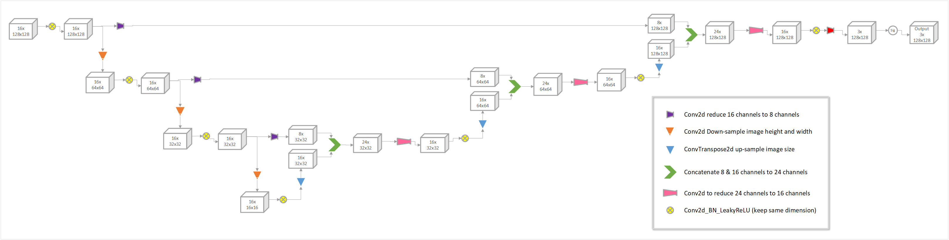
Figure 4 An example of network using Conv2d to achieve the desired output channels, height and width.
3. Implementation #1 of Conv2d forward and backward
In order to gain hands-on experience and full understanding of Conv2d, we implemented two versions of the Conv2d, both by subclassing torch.autograd.Function and manually overriding the forward and backward methods. The 1st version is kind of collection of multiple small modules including unfold, matrix multiplication, fold, etc. The 2nd version is more like brute force implementation of the equations using nested for loops.
To validate our custom implementations, we build a small Conv2d-LeakyReLU-Mean network and compared the outputs and autograd results with the Torch built-in implementation. The LeakyReLU layer is also custom implemented.
This section covers Version #1 and the compete source code can be found on GitHub (my_conv2d_v1.py).
3.1. Forward in Version #1
This implementation is inspired by the discussion of using unfold function here. The forward function is overridden to take 5 input arguments:
- ctx: represent THIS instance of the class
- inX: the 4-D input tensor with a shape of (nImgSamples, nInCh, nInImgRows, nInImgCols)
- in_weight: the 4-D learnable convolution kernel with a shape of (nOutCh, nInCh, nKnRows, nKnCols)
- in_bias: 1-D learnable convolution bias with a shape of (nOutCh,)
- convparam: tuple to pass in parameters of (padding, stride), default=(0,1)
The core part is listed below. For the convenience of tracking and readability, the name of each variable is a combination of its meaning and dimensions to indicate the shape of the tensor.
1.   inX_nSamp_nB_nL = torch.nn.functional.unfold(inX, (nKnRows, nKnCols), padding=padding, stride=stride)
2.   inX_nSamp_nL_nB = inX_nSamp_nB_nL.transpose(1, 2)
3.   kn_nOutCh_nB = in_weight.view(nOutCh, -1)
4.   kn_nB_nOutCh = kn_nOutCh_nB.t()
5.   out_nSamp_nL_nOutCh = inX_nSamp_nL_nB.matmul(kn_nB_nOutCh)
6.   out_nSamp_nOutCh_nL = out_nSamp_nL_nOutCh.transpose(1, 2)
7.   out = out_nSamp_nOutCh_nL.reshape(nImgSamples, nOutCh, nOutRows, nOutCols)
8.   if in_bias is not None:
9.      out += in_bias.view(1, -1, 1, 1)
Line 1: call the unfold function to extract nOutRows x nOutCols patches per sample from the input and each patch has a size of inChannels x nKnRows x nKnCols elements and can be multiplied with the convolution kernels. The input tensor has a shape of (nImgSamples, nInCh, nInImgRows, nInImgCols) and the unfold output tensor has a shape of (nImgSamples, nB=inChannels x nKnRows x nKnCols, nL=nOutRows X nOutCols).
Line 2-4: reshape the unfolded data and kernel to so that the last dimension of inX_nSamp_nL_nB and the first dimension of kn_nB_nOutCh have the same size (nB) for matrix multiplication.
Line 5: Apply matrix multiplication.
Line 6-7: Reshape the result to match the output shape.
Line 8: Add the bias, if specified, to obtain the final output from MyConv2d.
It returns a 4-D tensor of the convolution results with a shape of (nImgSamples, nOutCh, nOutRows, nOutCols).
3.2. Backward in Version #1
The backward function is overridden to take one argument (in addition to THIS instance ctx), which must match the output list of the forward function:
- grad_from_upstream: the 4-D tensor of the upstream gradient for the convolution. It has the same shape as the forward output, (nImgSamples, nOutCh, nOutRows, nOutCols)
The backward function must return the same number of items as the argument list of the forward function, not including ctx. More specifically, it must return 3 gradients of the loss w.r.t. to inX, in_weight and in_bias (if specified, otherwise a None) respectively, plus a None for convparam that is just a tuple of parameters and does not require gradient.
Please see the source code for detailed implementation and it is quite self-explanatory with comments above each step. In fact, it starts from the upstreaming gradient, using the chain rule as discussed in the previous posts, and computes the gradients of each step of the forward function in reversed order.
It is worth mentioning that, because inX_nSamp_nL_nB and kn_nB_nOutCh are involved in matrix multiplication, we used the conclusion from the previous post to calculate their gradients:
for the matrix multiplication of \( \boldsymbol {C} = \boldsymbol {A} \boldsymbol {B} \).
Another thing to note is that the fold function is called, like a counterpart of the unfold function used in the forward function, to sum and patch the intermediate gradient data grad_inX_nSamp_nB_nL back into the shape of inX, (nImgSamples, nInCh, nInImgRows, nInImgCols).
4. Implementation #2 of Conv2d forward and backward
The 2nd version of implementation of Conv2d has the same interfaces of the forward and backward function when subclassing torch.autograd.Function. Different from the 1st version that is a collection of multiple steps, the 2nd version directly implements the equations (1) and (2) using 3 nested for loops. Please see the complete source code of this implementation (my_conv2d_v2.py) on GitHub.
4.1. Forward in Version #2
The core part is listed below. For convenience of calculation, the input tensor inX is padded to a new bigger tensor paddedX. Inside the center of the 3 nested for loops, it is the element-wise multiplication of the input patch with the kernel, followed by the sum, which is exactly implementation of Equation (1).
paddedX[:,:,padding:nInImgRows+padding,padding:nInImgCols+padding] = inX

for outCh in range(nOutCh):
   for iRow in range(nOutRows):
      startRow = iRow * stride

      for iCol in range(nOutCols):
         startCol = iCol * stride

         out[:, outCh, iRow, iCol] = \
            (paddedX[:,:,startRow:startRow+nKnRows,startCol:startCol+nKnCols] \
            * in_weight[outCh,:,0:nKnRows,0:nKnCols]).sum(axis=(1,2,3))
Similarly to the 1st version, it returns a 4-D tensor of the convolution results with a shape of (nImgSamples, nOutCh, nOutRows, nOutCols).
4.2. Backward in Version #2
Again, the backward function must return 3 gradients of the loss w.r.t. to inX, in_weight and in_bias (if specified, otherwise a None) respectively, plus a None for convparam that is just a tuple of parameters and does not require gradient.
It uses the same 3 nested for loops to compute the gradients and the core part is listed below. Inside the center of the loops, it also follows the two key ideas of the backpropagation chain rule: 1) summation of all paths and 2) product of upstream and local gradients along each path. Pleate note that, in calculation of the gradients of the kernel (grad_weight), the results are summed with sum(axis=0) because the kernel is applied to all samples, which is the 1st dimension (axis=0). The same logic applies to grad_bias too.
for outCh in range(nOutCh):
   for iRow in range(nOutRows):
      startRow = iRow * stride

         for iCol in range(nOutCols):
            startCol = iCol * stride

            grad_padX[:,:,startRow:startRow+nKnRows,startCol:startCol+nKnCols] += \
               grad_from_upstream[:, outCh, iRow, iCol].reshape(-1, 1, 1, 1) * \
               in_weight[outCh, :, 0:nKnRows, 0:nKnCols]

            grad_weight[outCh, :, 0:nKnRows, 0:nKnCols] += \
               (paddedX[:,:,startRow:startRow+nKnRows,startCol:startCol+nKnCols] * \
               grad_from_upstream[:, outCh, iRow, iCol].reshape(-1, 1, 1, 1)).sum(axis=0)

grad_inputX = grad_padX[:,:,padding:nPadImgRows-padding,padding:nPadImgCols-padding]

if in_bias is not None:
   grad_bias = grad_from_upstream.sum(axis=(0, 2, 3))
5. Validation against Torch built-ins
To validate our custom implementations, we build a small Conv2d-LeakyReLU-Mean network (Figure 5) and compared the outputs and autograd results with the Torch built-in implementation[1]. The LeakyReLU layer is also custom implemented and the source code can be found here. The validation code can be found here. Results show that both implementations of Conv2d produced the same results as the Torch built-ins, including the output and the gradients w.r.t. the input, kernel and bias.
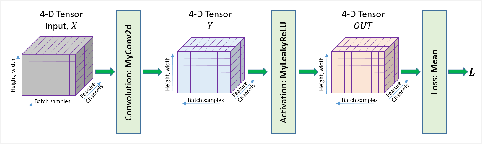
Figure 5 Illustration of Conv2d-LeakyReLU-Mean network used for validation.
6. Summary
In this post, we discussed the fundamentals of Conv2d and demonstrated how to implement its forward and backward autograd functions using 2 different ways. In the end, we built a simple Conv2d-LeakyReLU-Mean network to test our implementations. Only Conv2d is used as example, but all ideas can be extended to Conv1d and Conv3d. We hope that, by going through this example, it can help us obtain a deeper understanding of the convolution in neural networks. In next post, we will move to ConvTranpose.
7. Extra – Edge detection and smoothing using pre-defined kernels
While the convolution kernel and bias in neural networks are learnable parameters, standalone Conv2d can also be used to perform specific tasks using pre-defined kernels. In this section, we would like to demonstrate two applications of Conv2d: edge detection and smoothing. In both examples, we use the same input image as shown in Figure 6.

Figure 6 The original image of leaves.
7.1. Sobel edge detection using Conv2d
Sobel filter[2] is used in this example to demonstrate application of Conv2d in edge detection tasks. Two 3x3 Sobel kernels are given by
For a 2-D input image \( \boldsymbol {I} \), the Sobel edge detection output image \( \boldsymbol {O} \) is given by
The source code can be found here and the output image is shown in Figure 7.
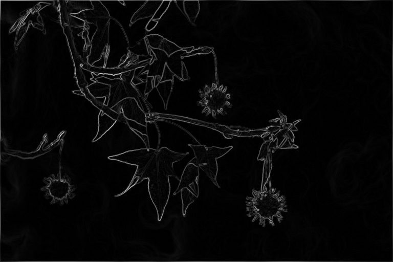
Figure 7 The Sobel edge detection output image.
7.2. Gaussian blurring using Conv2d
A normalized 5x5 Gaussian kernel is given by
For a 2-D input image \( \boldsymbol {I} \), the Gaussian blurred output image \( \boldsymbol {O} \) is given by
The source code can be found here and the blurred output image is shown in Figure 8.
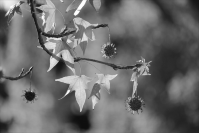
Figure 8 The the Gaussian blurred output image.